
The goal of revpref is to provide a set of tools to (i)
check consistency of a finite set of consumer demand observations with a
number of revealed preference axioms at a given efficiency level, (ii)
compute goodness-of-fit indices when the data do not obey the axioms,
and (iii) compute power against uniformly random behavior. Below we
provide a brief description of the functions provided in this
package.
Nonparametric tests to check whether the data set is consistent with the revealed preference axioms at any efficiency level
warp tests consistency with the Weak Axiom of
Revealed Preference (WARP) at efficiency level e and reports the number
of WARP violations.
sarp tests consistency with the Strong Axiom of
Revealed Preference (SARP) at efficiency level e and reports the number
of SARP violations.
garp tests consistency with the Generalized Axiom of
Revealed Preference (GARP) at efficiency level e and reports the number
of GARP violations.
Note: for all the three functions described above
(warp, sarp, and garp), the user
must provide a T X N price matrix and a T X N quantity matrix where T
corresponds to the number of observations and N corresponds to the
number of consumption categories. Further, all prices are required to be
strictly positive. Optionally, the efficiency level e at which the user
would like to test consistency with the axiom(s) can also be provided.
When e is not specified, it defaults to 1, which checks consistency with
the exact axiom(s).
For a comprehensive overview of the theory of revealed preferences, see Varian (2006) and Cherchye et al. (2009).
Goodness-of-fit to measure the severity of violations
ccei computes the critical cost efficiency index,
CCEI (also known as the Afriat efficiency index). The CCEI is defined as
the maximal value of the efficiency level e at which the data set is
consistent with GARP. Intuitively, this measure indicates the degree to
which the set of demand observations is consistent with GARP. The user
needs to provide a T X N price matrix and a T X N quantity matrix where
T corresponds to the number of observations and N corresponds to the
number of consumption categories. Optionally, the user can specify the
axiom (WARP, SARP, or GARP) for which the CCEI needs to be computed.
When no axiom is specified, the function takes the default option as
GARP.
mpi computes the minimum and maximum money pump
index (MPI). Echenique et al. (2011) proposed the money pump index as a
measure of the severity of GARP violation. It is defined as the amount
of money that an arbitrageur can “pump” from the consumer. While the MPI
measure is conceptually appealing, it may be computationally challenging
to determine this index for data sets with a large number of
observations. In particular, Smeulders et al. (2013) showed that
computing the mean and median MPI is an NP-hard problem. As
easy-to-apply alternatives, Smeulders et al. (2013) proposed the minimum
and maximum MPIs which can be computed efficiently (in polynomial time).
The function mpi implements the algorithm provided by these
authors to compute the minimum and maximum MPI values for the given
data.
Power of the revealed preference tests
bronars computes the Bronars power index which is
defined as the probability of rejecting a given rationality axiom
provided that the data is defined by irrational behavior (Bronars
(1987)). Following Bronars’ (1987) suggestion, we use Becker’s
bronars computes the Bronars power index for any
of the three axioms (WARP, SARP, or GARP) at any efficiency level.You can install the released version of revpref from CRAN with:
install.packages("revpref")And the development version from GitHub with:
# install.packages("devtools")
devtools::install_github("ksurana21/revpref")Below we provide some simple examples to illustrate the three types of functionality available within the package. To begin with, we define the price and quantity matrices. Both of these matrices (defined below) have ten rows corresponding to the number of observations and three columns corresponding to the number of consumption categories.
# Load the package
library(revpref)

# Define a price matrix
p = matrix(c(4, 4, 4, 1, 9, 3, 2, 8, 3, 1,
             8, 4, 3, 1, 9, 3, 2, 8, 8, 4,
             1, 4, 1, 8, 9, 3, 1, 8, 3, 2),
           nrow = 10, ncol = 3, byrow = TRUE)

# Define a quantity matrix
q = matrix(c( 01.81, 00.19, 10.51, 17.28, 02.26, 04.13, 12.33, 02.05, 02.99, 06.06,
              05.19, 00.62, 11.34, 10.33, 00.63, 04.33, 08.08, 02.61, 04.36, 01.34,
              09.76, 01.37, 36.35, 01.02, 03.21, 04.97, 06.20, 00.32, 08.53, 10.92),
           nrow = 10, ncol = 3, byrow = TRUE)
Nonparametric tests
First, we check whether the data violate the rationality axioms. We begin with GARP.
# Test consistency with GARP and compute the number of GARP violations
result <- garp(p, q)
result
#> [1] 0 8
The first output is a binary indicator telling us whether the data set passed the GARP test. Here, we see that the first output is 0 which means that the data set is inconsistent with GARP. The second output indicates that there are 8 GARP violations. In this example, we did not specify the efficiency level, in which case the default value of 1 was applied. In the next example, we check GARP at the efficiency level e = 0.90.
# Test consistency with GARP and compute the number of violations at the efficiency level 0.90
result <- garp(p, q, efficiency = 0.90)
result
#> [1] 1 0
Here we see that the first output is 1 which means that the data set is consistent with GARP at the efficiency level e = 0.90. As expected, the second output is 0 indicating that there are no GARP violations at this efficiency level. Next, we follow similar procedures to test consistency with SARP and WARP at full efficiency.
# Test consistency with SARP and compute the number of SARP violations
result <- sarp(p, q)
result
#> [1] 0 8

# Test consistency with WARP and compute the number of WARP violations
result <- warp(p, q)
result
#> [1] 0 1
We see that the data set is inconsistent with both SARP and WARP. All the three tests revealed that our data set failed to satisfy the rationality axioms. However, these tests did not indicate how close this set of observations is to satisfying the exact axioms. In the next step, we compute goodness-of-fit indices to measure the severity of violations.
Goodness-of-fit
The package provides functionalities for two goodness-of-fit measures. The first measure is the critical cost efficiency index (CCEI) which is defined as the maximal efficiency level at which the data set is consistent with the rationality axiom(s). From the previous exercises, we know that our data set failed to satisfy GARP at full efficiency but is consistent with GARP at the efficiency level 0.90. As such, we expect the CCEI to be greater than 0.90 but less than 1.
# Compute the Critical Cost Efficiency Index (CCEI)
result <- ccei(p, q)
result
#> [1] 0.9488409
Using the function ccei, we find that the highest
efficiency level at which the data set is consistent with GARP is equal
to 0.9488. This indicates that although our data set is inconsistent
with the exact GARP, it is very close to satisfying it. We can also
compute the CCEI for SARP and WARP by providing an additional argument
(model = “SARP” or model = “WARP”).
# Compute the Critical Cost Efficiency Index (CCEI) for SARP
result <- ccei(p, q, model = "SARP")
result
#> [1] 0.9488409
The second goodness-of-fit measure which can be computed through this
package is the money pump index (MPI). We can compute the minimum and
maximum MPI using the function mpi as follows,
# Compute the minimum and maximum Money Pump Index (MPI)
result <- mpi(p, q)
result
#> [1] 0.07242757 0.18732824
The output tells us that the minimum and maximum MPIs for this data set are 0.07243 and 0.1873, respectively. This means that the consumer is losing 7.24% of the budget in the least severe violation and 18.73% of the budget in the most severe violation. Implicitly, these values provide a bound on the amounts of money that can be pumped from this consumer.
Power
In addition to goodness-of-fit measures, empirical studies usually
also report the power measure. As discussed above, the power of a
revealed preference test is a measure of the likelihood of detecting an
irrational behavior. We can use the function bronars to
compute the Bronars power index for the given data set.
# Compute power
result <- bronars(p, q)
result
#> [1] 0.839
We find that for the given budget conditions, there is about 83.90% probability of detecting irrational behavior. As discussed above, here we have followed Becker’s (1962) approach of using uniformly random consumption choices to simulate irrational consumers. As a final exercise, we analyze how the power of the GARP test changes with the efficiency level.
# Compute power of the GARP test at efficiency levels between 0.4 to 1
power <- c()
for(i in seq(0.4, 1, by = 0.05)){
  power = rbind(power, c(i, bronars(p, q, model = "GARP", simulation = 1000,
                                    efficiency = i)))
}

# Plot the power measures against efficiency levels
power <- as.data.frame(power)
names(power) <- c("efficiency", "power")
plot(power, type = "b",col = "black", lwd = 1, pch = 20, bty = "L")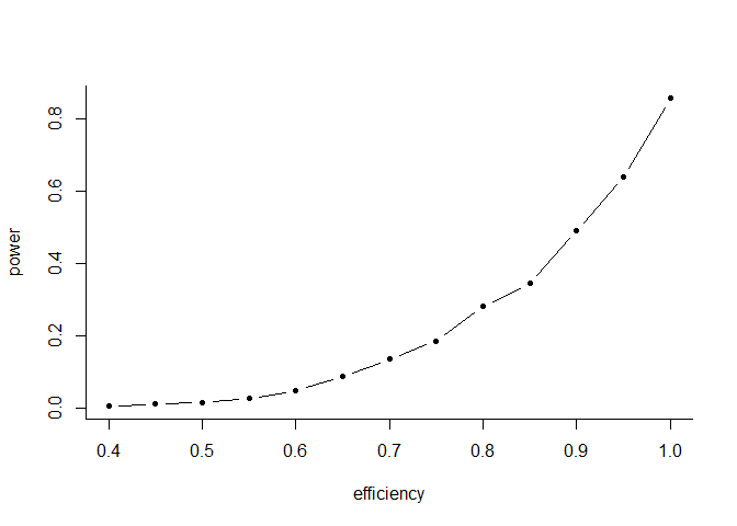
As depicted in the figure above, the power of the GARP test increases with the efficiency level. This is expected as the lower is the efficiency level, the weaker is the test. In other words, with lower values of efficiency, a larger fraction of the simulated data is able to pass the test and hence the probability of rejecting GARP is smaller.
Becker, Gary S. “Irrational behavior and economic theory.” Journal of political economy 70, no. 1 (1962): 1-13.
Bronars, Stephen G. “The power of nonparametric tests of preference maximization.” Econometrica: Journal of the Econometric Society (1987): 693-698.
Cherchye, Laurens, Ian Crawford, Bram De Rock, and Frederic Vermeulen. “The revealed preference approach to demand.” In Quantifying Consumer Preferences. Emerald Group Publishing Limited,
Echenique, Federico, Sangmok Lee, and Matthew Shum. “The money pump as a measure of revealed preference violations.” Journal of Political Economy 119, no. 6 (2011): 1201-1223.
Smeulders, Bart, Laurens Cherchye, Frits CR Spieksma, and Bram De Rock. “The money pump as a measure of revealed preference violations: A comment.” Journal of Political Economy 121, no. 6 (2013): 1248-1258.
Varian, Hal R. “Revealed preference.” Samuelsonian economics and the twenty-first century (2006): 99-115.