
![]()
mpoly is a simple collection of tools to help deal
with multivariate polynomials symbolically and functionally in
R. Polynomials are defined with the mp() function:
library("mpoly")
mp("x + y")
# x  +  y

mp("(x + 4 y)^2 (x - .25)")
# x^3  -  0.25 x^2  +  8 x^2 y  -  2 x y  +  16 x y^2  -  4 y^2
Term orders are available with the reorder function:
(p <- mp("(x + y)^2 (1 + x)"))
# x^3  +  x^2  +  2 x^2 y  +  2 x y  +  x y^2  +  y^2

reorder(p, varorder = c("y","x"), order = "lex")
# y^2 x  +  y^2  +  2 y x^2  +  2 y x  +  x^3  +  x^2

reorder(p, varorder = c("x","y"), order = "glex")
# x^3  +  2 x^2 y  +  x y^2  +  x^2  +  2 x y  +  y^2
Vectors of polynomials (mpolyList’s) can be specified in
the same way:
mp(c("(x+y)^2", "z"))
# x^2  +  2 x y  +  y^2
# zYou can extract pieces of polynoimals using the standard
[ operator, which works on its terms:
p[1]
# x^3

p[1:3]
# x^3  +  x^2  +  2 x^2 y

p[-1]
# x^2  +  2 x^2 y  +  2 x y  +  x y^2  +  y^2
There are also many other functions that can be used to piece apart polynomials, for example the leading term (default lex order):
LT(p)
# x^3

LC(p)
# [1] 1

LM(p)
# x^3
You can also extract information about exponents:
exponents(p)
# [[1]]
# x y
# 3 0
#
# [[2]]
# x y
# 2 0
#
# [[3]]
# x y
# 2 1
#
# [[4]]
# x y
# 1 1
#
# [[5]]
# x y
# 1 2
#
# [[6]]
# x y
# 0 2

multideg(p)
# x y
# 3 0

totaldeg(p)
# [1] 3

monomials(p)
# x^3
# x^2
# 2 x^2 y
# 2 x y
# x y^2
# y^2Arithmetic is defined for both polynomials (+,
-, * and ^)…
p1 <- mp("x + y")

p2 <- mp("x - y")

p1 + p2
# 2 x

p1 - p2
# 2 y

p1 * p2
# x^2  -  y^2

p1^2
# x^2  +  2 x y  +  y^2
… and vectors of polynomials:
(ps1 <- mp(c("x", "y")))
# x
# y

(ps2 <- mp(c("2 x", "y + z")))
# 2 x
# y  +  z

ps1 + ps2
# 3 x
# 2 y  +  z

ps1 - ps2
# -1 x
# -1 z

ps1 * ps2
# 2 x^2
# y^2 + y zYou can compute derivatives easily:
p <- mp("x + x y + x y^2")

deriv(p, "y")
# x  +  2 x y

gradient(p)
# y^2  +  y  +  1
# 2 y x + xYou can turn polynomials and vectors of polynomials into functions
you can evaluate with as.function(). Here’s a basic example
using a single multivariate polynomial:
f <- as.function(mp("x + 2 y")) # makes a function with a vector argument
# f(.) with . = (x, y)

f(c(1,1))
# [1] 3

f <- as.function(mp("x + 2 y"), vector = FALSE) # makes a function with all arguments
# f(x, y)

f(1, 1)
# [1] 3
Here’s a basic example with a vector of multivariate polynomials:
(p <- mp(c("x", "2 y")))
# x
# 2 y

f <- as.function(p)
# f(.) with . = (x, y)

f(c(1,1))
# [1] 1 2

f <- as.function(p, vector = FALSE)
# f(x, y)

f(1, 1)
# [1] 1 2
Whether you’re working with a single multivariate polynomial or a
vector of them (mpolyList), if it/they are actually
univariate polynomial(s), the resulting function is vectorized. Here’s
an example with a single univariate polynomial.
f <- as.function(mp("x^2"))
# f(.) with . = x

f(1:3)
# [1] 1 4 9

(mat <- matrix(1:4, 2))
#      [,1] [,2]
# [1,]    1    3
# [2,]    2    4

f(mat) # it's vectorized properly over arrays
#      [,1] [,2]
# [1,]    1    9
# [2,]    4   16
Here’s an example with a vector of univariate polynomials:
(p <- mp(c("t", "t^2")))
# t
# t^2

f <- as.function(p)
f(1)
# [1] 1 1

f(1:3)
#      [,1] [,2]
# [1,]    1    1
# [2,]    2    4
# [3,]    3    9
You can use this to visualize a univariate polynomials like this:
library("tidyverse"); theme_set(theme_classic())f <- as.function(mp("(x-2) x (x+2)"))
# f(.) with . = x
x <- seq(-2.5, 2.5, .1)
qplot(x, f(x), geom = "line")
# Warning: `qplot()` was deprecated in ggplot2 3.4.0.
# This warning is displayed once every 8 hours.
# Call `lifecycle::last_lifecycle_warnings()` to see where this warning was
# generated.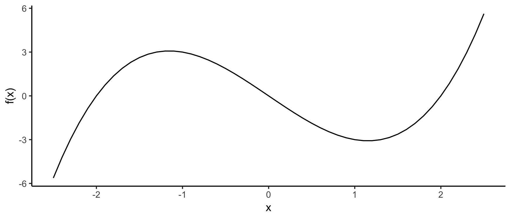
For multivariate polynomials, it’s a little more complicated:
f <- as.function(mp("x^2 - y^2"))
# f(.) with . = (x, y)
s <- seq(-2.5, 2.5, .1)
df <- expand.grid(x = s, y = s)
df$f <- apply(df, 1, f)
qplot(x, y, data = df, geom = "raster", fill = f)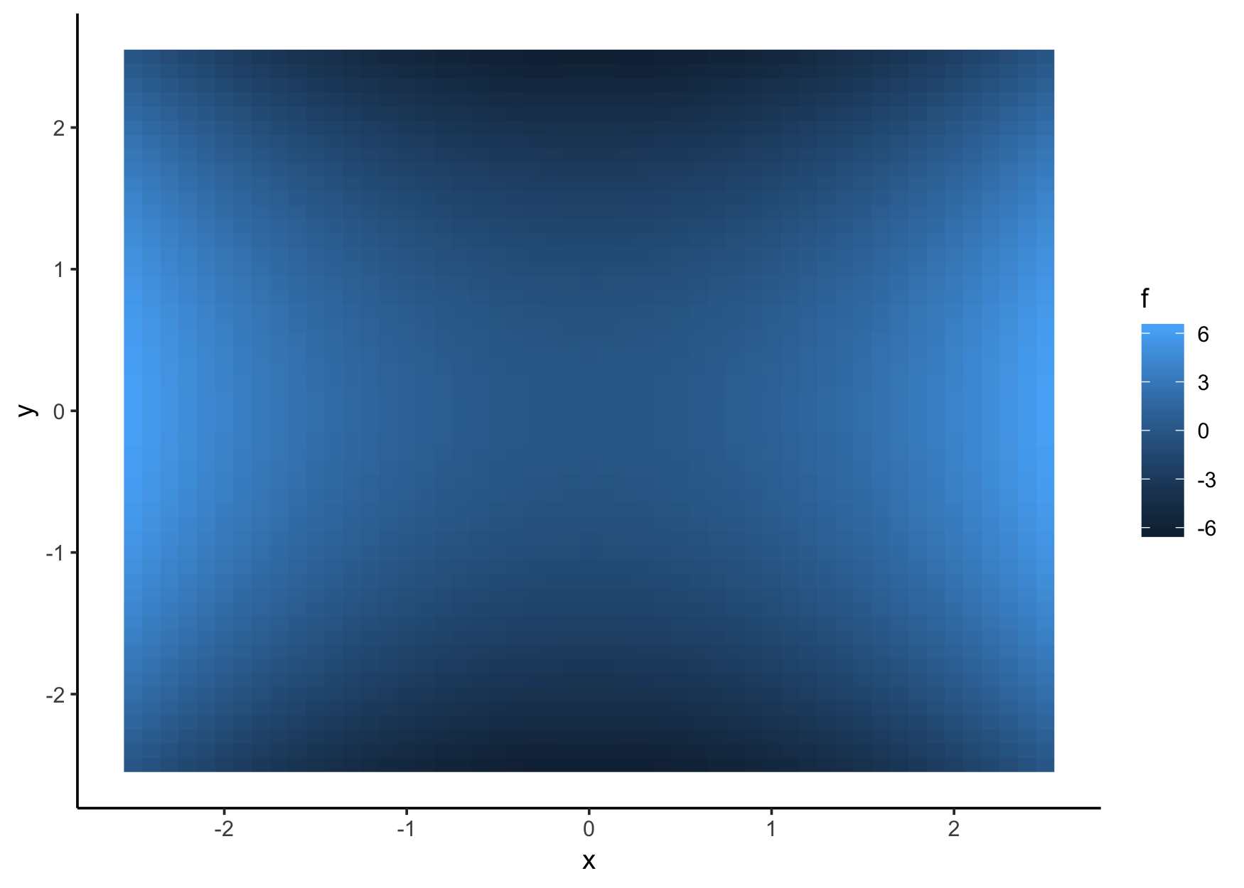
Using tidyverse-style coding
(install tidyverse packages with
install.packages("tidyverse")), this looks a bit
cleaner:
f <- as.function(mp("x^2 - y^2"), vector = FALSE)
# f(x, y)
seq(-2.5, 2.5, .1) %>%
  list("x" = ., "y" = .) %>%
  cross_df() %>%
  mutate(f = f(x, y)) %>%
  ggplot(aes(x, y, fill = f)) +
    geom_raster()
# Warning: `cross_df()` was deprecated in purrr 1.0.0.
# ℹ Please use `tidyr::expand_grid()` instead.
# ℹ See <https://github.com/tidyverse/purrr/issues/768>.
# This warning is displayed once every 8 hours.
# Call `lifecycle::last_lifecycle_warnings()` to see where this warning was
# generated.
Grobner bases are no longer implemented in mpoly; they’re now in m2r.
# polys <- mp(c("t^4 - x", "t^3 - y", "t^2 - z"))
# grobner(polys)
Homogenization and dehomogenization:
(p <- mp("x + 2 x y + y - z^3"))
# x  +  2 x y  +  y  -  z^3

(hp <- homogenize(p))
# x t^2  +  2 x y t  +  y t^2  -  z^3

dehomogenize(hp, "t")
# x  +  2 x y  +  y  -  z^3

homogeneous_components(p)
# x  +  y
# 2 x y
# -1 z^3mpoly can make use of many pieces of the
polynom and orthopolynom packages with
as.mpoly() methods. In particular, many special polynomials
are available.
You can construct Chebyshev polynomials as follows:
chebyshev(1)
# x

chebyshev(2)
# -1  +  2 x^2

chebyshev(0:5)
# 1
# x
# 2 x^2  -  1
# 4 x^3  -  3 x
# 8 x^4  -  8 x^2  +  1
# 16 x^5  -  20 x^3  +  5 x
And you can visualize them:
s <- seq(-1, 1, length.out = 201); N <- 5
(chebPolys <- chebyshev(0:N))
# 1
# x
# 2 x^2  -  1
# 4 x^3  -  3 x
# 8 x^4  -  8 x^2  +  1
# 16 x^5  -  20 x^3  +  5 x

df <- as.function(chebPolys)(s) %>% cbind(s, .) %>% as.data.frame()
names(df) <- c("x", paste0("T_", 0:N))
mdf <- df %>% gather(degree, value, -x)
qplot(x, value, data = mdf, geom = "path", color = degree)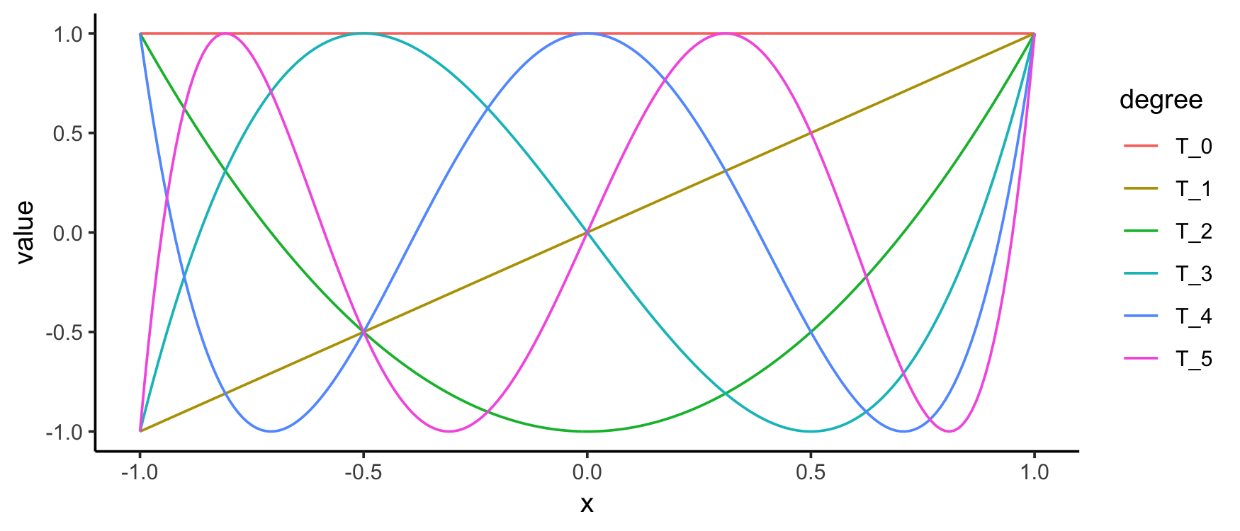
s <- seq(-1, 1, length.out = 201); N <- 5
(jacPolys <- jacobi(0:N, 2, 2))
# 1
# 5 x
# 17.5 x^2  -  2.5
# 52.5 x^3  -  17.5 x
# 144.375 x^4  -  78.75 x^2  +  4.375
# 375.375 x^5  -  288.75 x^3  +  39.375 x

df <- as.function(jacPolys)(s) %>% cbind(s, .) %>% as.data.frame
names(df) <- c("x", paste0("P_", 0:N))
mdf <- df %>% gather(degree, value, -x)
qplot(x, value, data = mdf, geom = "path", color = degree) +
  coord_cartesian(ylim = c(-25, 25))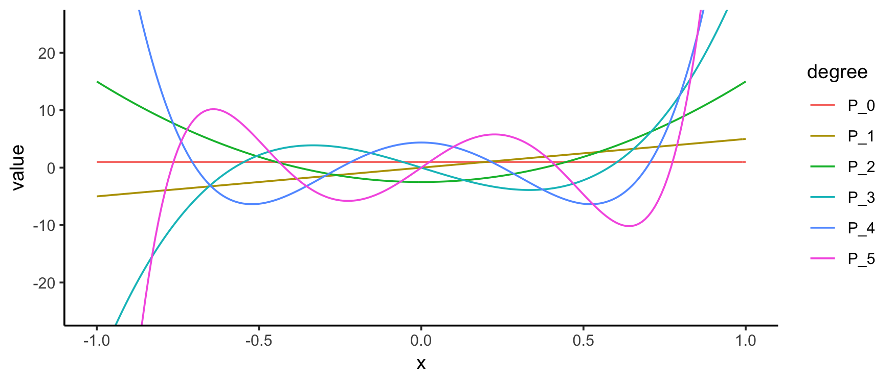
s <- seq(-1, 1, length.out = 201); N <- 5
(legPolys <- legendre(0:N))
# 1
# x
# 1.5 x^2  -  0.5
# 2.5 x^3  -  1.5 x
# 4.375 x^4  -  3.75 x^2  +  0.375
# 7.875 x^5  -  8.75 x^3  +  1.875 x

df <- as.function(legPolys)(s) %>% cbind(s, .) %>% as.data.frame
names(df) <- c("x", paste0("P_", 0:N))
mdf <- df %>% gather(degree, value, -x)
qplot(x, value, data = mdf, geom = "path", color = degree)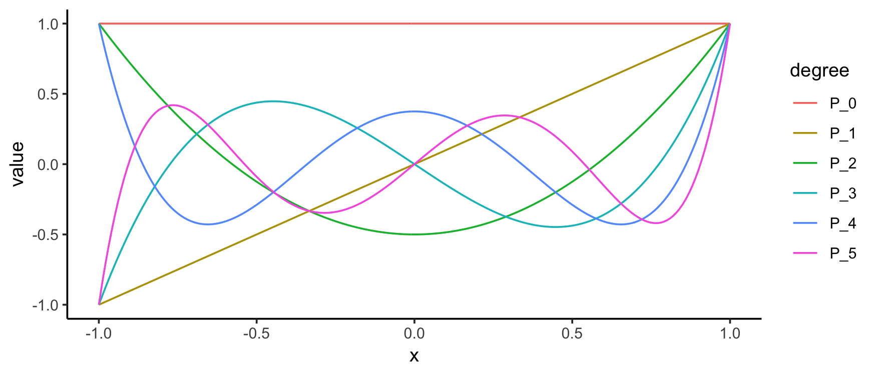
s <- seq(-3, 3, length.out = 201); N <- 5
(hermPolys <- hermite(0:N))
# 1
# x
# x^2  -  1
# x^3  -  3 x
# x^4  -  6 x^2  +  3
# x^5  -  10 x^3  +  15 x

df <- as.function(hermPolys)(s) %>% cbind(s, .) %>% as.data.frame
names(df) <- c("x", paste0("He_", 0:N))
mdf <- df %>% gather(degree, value, -x)
qplot(x, value, data = mdf, geom = "path", color = degree)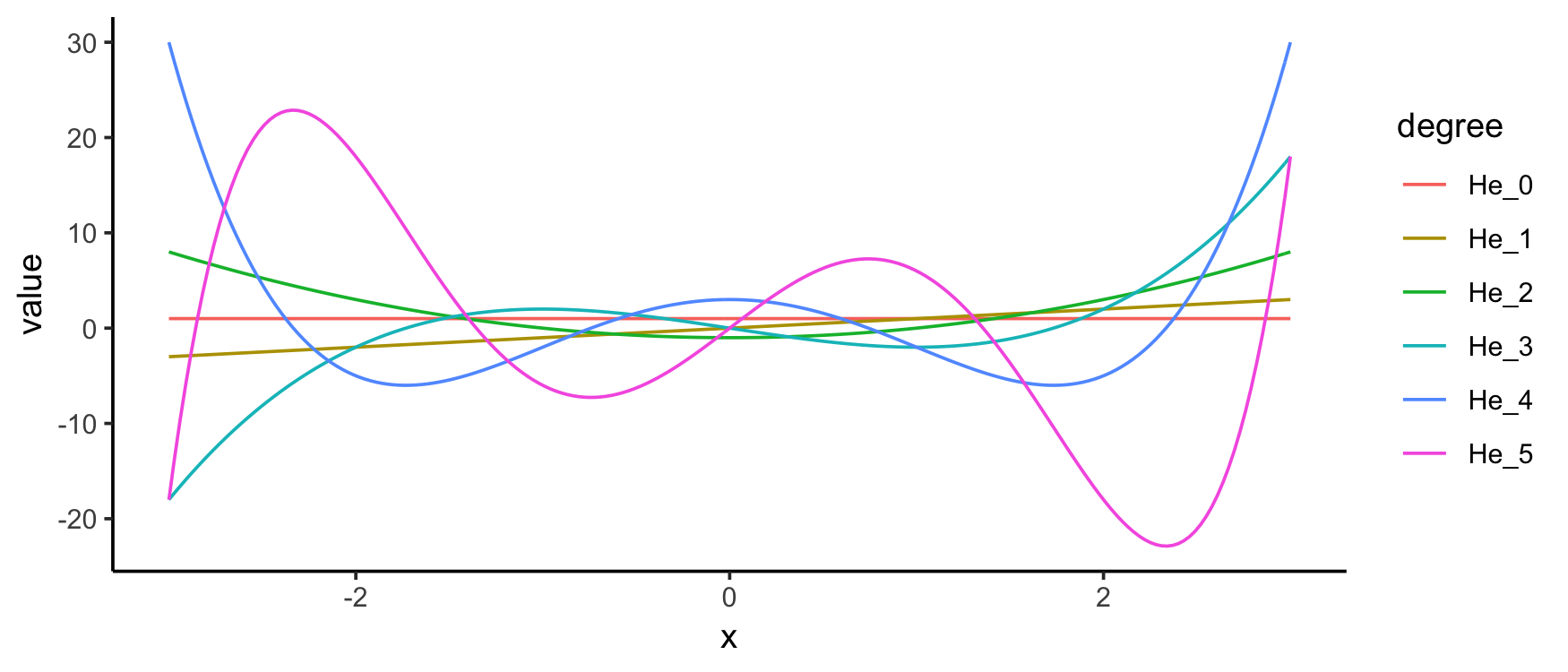
s <- seq(-5, 20, length.out = 201); N <- 5
(lagPolys <- laguerre(0:N))
# 1
# -1 x  +  1
# 0.5 x^2  -  2 x  +  1
# -0.1666667 x^3  +  1.5 x^2  -  3 x  +  1
# 0.04166667 x^4  -  0.6666667 x^3  +  3 x^2  -  4 x  +  1
# -0.008333333 x^5  +  0.2083333 x^4  -  1.666667 x^3  +  5 x^2  -  5 x  +  1

df <- as.function(lagPolys)(s) %>% cbind(s, .) %>% as.data.frame
names(df) <- c("x", paste0("L_", 0:N))
mdf <- df %>% gather(degree, value, -x)
qplot(x, value, data = mdf, geom = "path", color = degree) +
  coord_cartesian(ylim = c(-25, 25))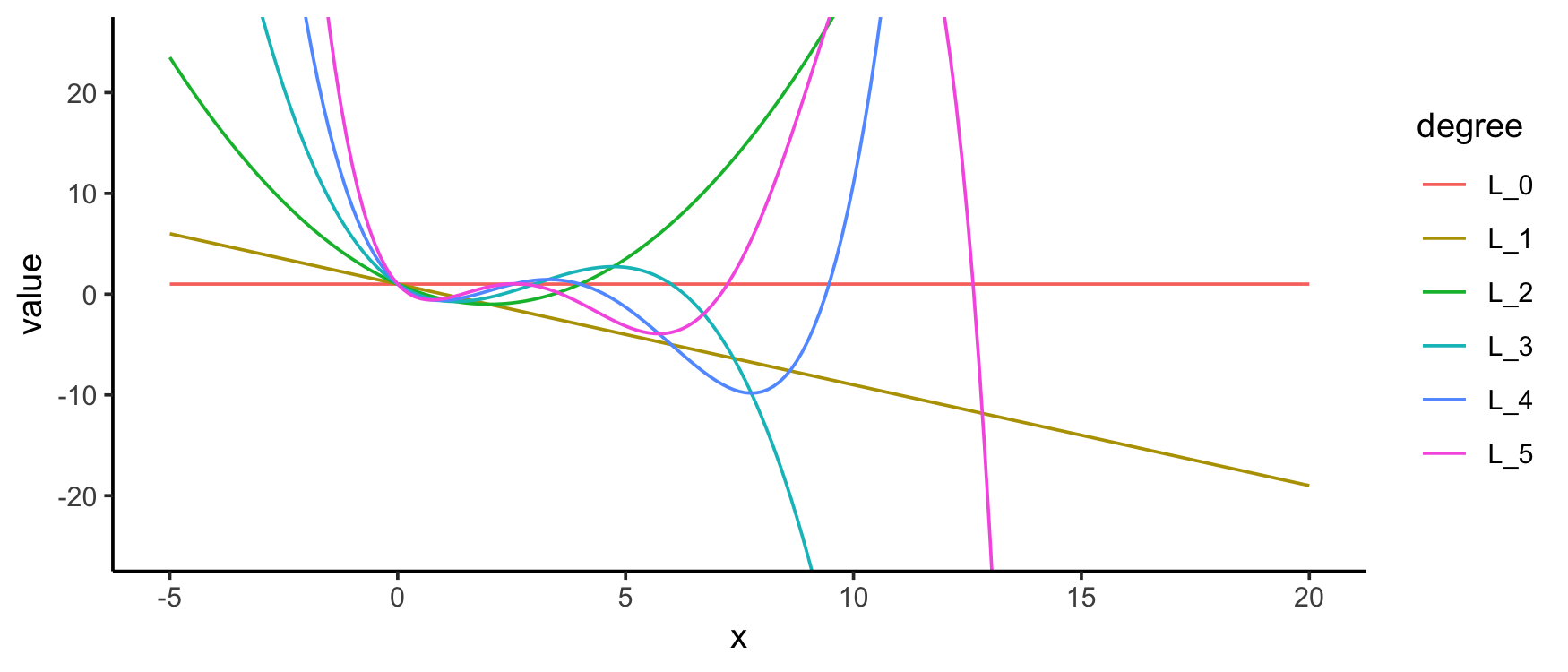
Bernstein
polynomials are not in polynom or
orthopolynom but are available in
mpoly with bernstein():
bernstein(0:4, 4)
# x^4  -  4 x^3  +  6 x^2  -  4 x  +  1
# -4 x^4  +  12 x^3  -  12 x^2  +  4 x
# 6 x^4  -  12 x^3  +  6 x^2
# -4 x^4  +  4 x^3
# x^4

s <- seq(0, 1, length.out = 101)
N <- 5 # number of bernstein polynomials to plot
(bernPolys <- bernstein(0:N, N))
# -1 x^5  +  5 x^4  -  10 x^3  +  10 x^2  -  5 x  +  1
# 5 x^5  -  20 x^4  +  30 x^3  -  20 x^2  +  5 x
# -10 x^5  +  30 x^4  -  30 x^3  +  10 x^2
# 10 x^5  -  20 x^4  +  10 x^3
# -5 x^5  +  5 x^4
# x^5

df <- as.function(bernPolys)(s) %>% cbind(s, .) %>% as.data.frame
names(df) <- c("x", paste0("B_", 0:N))
mdf <- df %>% gather(degree, value, -x)
qplot(x, value, data = mdf, geom = "path", color = degree)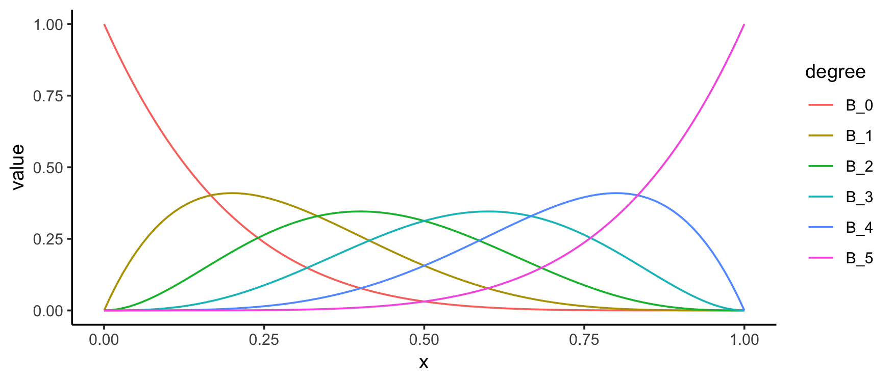
You can use the bernstein_approx() function to compute
the Bernstein polynomial approximation to a function. Here’s an
approximation to the standard normal density:
p <- bernstein_approx(dnorm, 15, -1.25, 1.25)
round(p, 4)
# -0.1624 x^2  +  0.0262 x^4  -  0.002 x^6  +  0.0001 x^8  +  0.3796

x <- seq(-3, 3, length.out = 101)
df <- data.frame(
  x = rep(x, 2),
  y = c(dnorm(x), as.function(p)(x)),
  which = rep(c("actual", "approx"), each = 101)
)
# f(.) with . = x
qplot(x, y, data = df, geom = "path", color = which)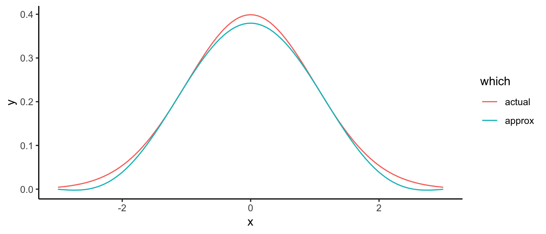
You can construct Bezier polynomials
for a given collection of points with bezier():
points <- data.frame(x = c(-1,-2,2,1), y = c(0,1,1,0))
(bezPolys <- bezier(points))
# -10 t^3  +  15 t^2  -  3 t  -  1
# -3 t^2  +  3 t
And viewing them is just as easy:
df <- as.function(bezPolys)(s) %>% as.data.frame

ggplot(aes(x = x, y = y), data = df) +
  geom_point(data = points, color = "red", size = 4) +
  geom_path(data = points, color = "red", linetype = 2) +
  geom_path(size = 2)
# Warning: Using `size` aesthetic for lines was deprecated in ggplot2 3.4.0.
# ℹ Please use `linewidth` instead.
# This warning is displayed once every 8 hours.
# Call `lifecycle::last_lifecycle_warnings()` to see where this warning was
# generated.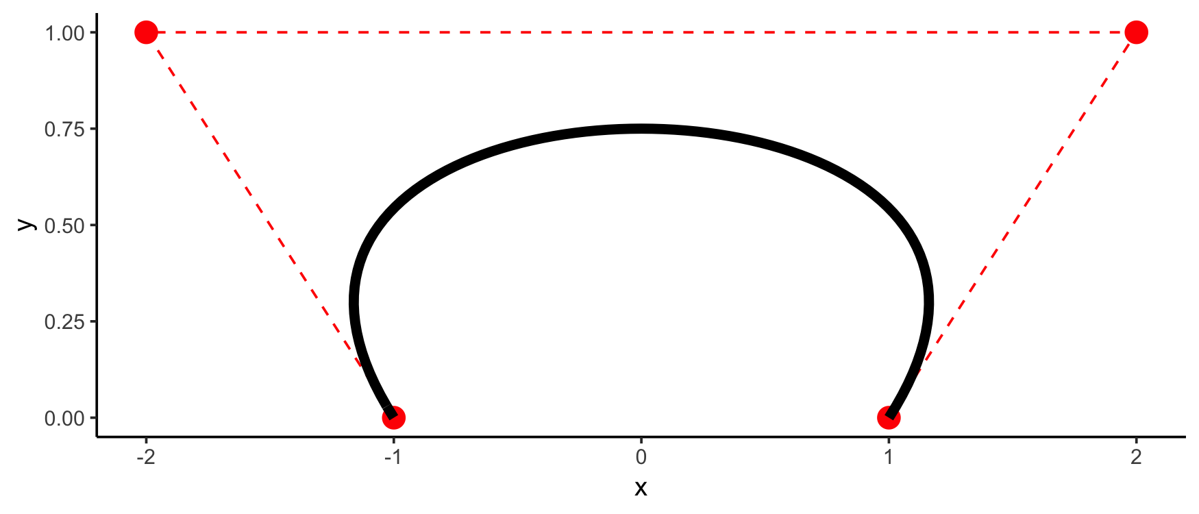
Weighting is available also:
points <- data.frame(x = c(1,-2,2,-1), y = c(0,1,1,0))
(bezPolys <- bezier(points))
# -14 t^3  +  21 t^2  -  9 t  +  1
# -3 t^2  +  3 t
df <- as.function(bezPolys, weights = c(1,5,5,1))(s) %>% as.data.frame

ggplot(aes(x = x, y = y), data = df) +
  geom_point(data = points, color = "red", size = 4) +
  geom_path(data = points, color = "red", linetype = 2) +
  geom_path(size = 2)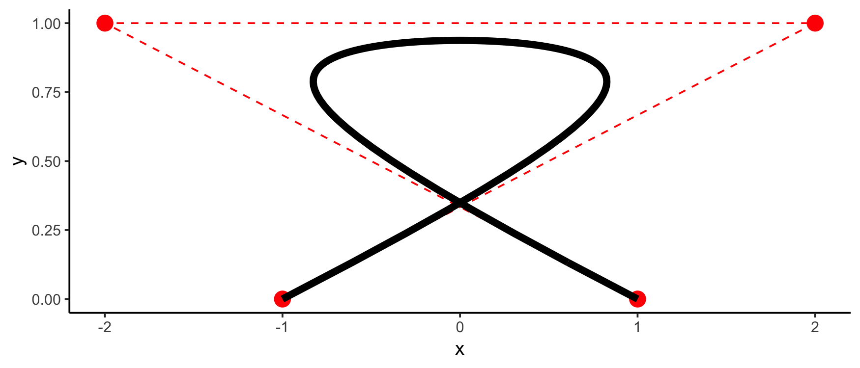
To make the evaluation of the Bezier polynomials stable,
as.function() has a special method for Bezier polynomials
that makes use of de
Casteljau’s algorithm. This allows bezier() to be used
as a smoother:
s <- seq(0, 1, length.out = 201)
df <- as.function(bezier(cars))(s) %>% as.data.frame
qplot(speed, dist, data = cars) +
  geom_path(data = df, color = "red")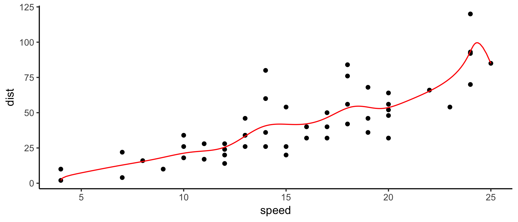
I’m starting to put in methods for some other R functions:
set.seed(1)
n <- 101
df <- data.frame(x = seq(-5, 5, length.out = n))
df$y <- with(df, -x^2 + 2*x - 3 + rnorm(n, 0, 2))

mod <- lm(y ~ x + I(x^2), data = df)
(p <- mod %>% as.mpoly %>% round)
# 1.983 x  -  1.01 x^2  -  2.709
qplot(x, y, data = df) +
  stat_function(fun = as.function(p), colour = 'red')
# f(.) with . = x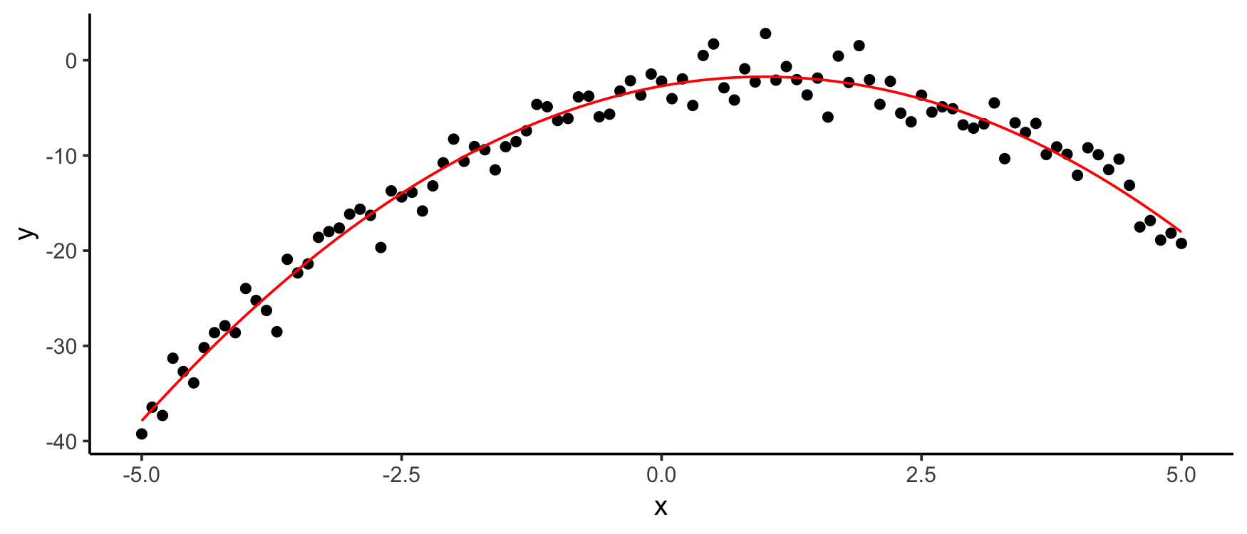
s <- seq(-5, 5, length.out = n)
df <- expand.grid(x = s, y = s) %>%
  mutate(z = x^2 - y^2 + 3*x*y + rnorm(n^2, 0, 3))

(mod <- lm(z ~ poly(x, y, degree = 2, raw = TRUE), data = df))
#
# Call:
# lm(formula = z ~ poly(x, y, degree = 2, raw = TRUE), data = df)
#
# Coefficients:
#                           (Intercept)  poly(x, y, degree = 2, raw = TRUE)1.0
#                             -0.070512                              -0.004841
# poly(x, y, degree = 2, raw = TRUE)2.0  poly(x, y, degree = 2, raw = TRUE)0.1
#                              1.005307                               0.001334
# poly(x, y, degree = 2, raw = TRUE)1.1  poly(x, y, degree = 2, raw = TRUE)0.2
#                              3.003755                              -0.999536
as.mpoly(mod)
# -0.004840798 x + 1.005307 x^2 + 0.001334122 y + 3.003755 x y - 0.9995356 y^2 - 0.07051218From CRAN: install.packages("mpoly")
From Github (dev version):
# install.packages("devtools")
devtools::install_github("dkahle/mpoly")This material is based upon work partially supported by the National Science Foundation under Grant No. 1622449.