In the course of a genome-wide association study, the situation often arises that some phenotypes are known with greater precision than others. It could be that some individuals are known to harbor more micro-environmental variance than others. In the case of inbred strains of model organisms, it could be the case that more organisms were observed from some strains than others, so the strains with more organisms have better-estimated means.
Package wISAM handles this situation by allowing for
weighting of each observation accoding to residual variance.
Specifically, the weight parameter to the function
conduct_scan takes the precision of each observation (one
over the variance).
You can install wISAM from github with:
install.packages("devtools")
devtools::install_github('rcorty/wISAM')
or from CRAN with:
install.packages('wISAM')Load the package and the example data will be available
automatically. You may want to have a look at the data format and shape
with str(). Create a standard genome scan (gs,
below) or one that uses weights (wgs, below). You can see
that this package uses a reference
class to implement the GenomeScan object.
library(wISAM)

gs <- GenomeScan$new(y = phenotype, X = covariate_mat, G = locus_list, K = kinship_mat)
wgs <- GenomeScan$new(y = phenotype, X = covariate_mat, G = locus_list, K = kinship_mat, w = 1/se_mean_per_strain)
You can then call prep_scan, which computes the
quantities that will only need to be computed once in the course of the
genome scan. Depending on the size of the population, this can be quite
slow. The methods of the GenomeScan reference class return the instance,
so you can chain them together. Unfortunately, this means you will need
to wrap the calls in invisible, or save them to an object to avoid
getting a big print to screen.
invisible(gs$prep_scan())
#> Preparing GenomeScan...
invisible(wgs$prep_scan())
#> Preparing GenomeScan...
You may want to investigate what changed in gs and
wgs when you ran prep_scan(). The next step is
to conduct the genome scan.
invisible(gs$conduct_scan())
#> Conducting GenomeScan...
invisible(wgs$conduct_scan())
#> Conducting GenomeScan...
After conducting a scan, you can have a look at the output.
plot(x = gs$Results$LR, col = c('red', rep('black', 99)))
plot(x = wgs$Results$LR, col = c('red', rep('black', 99)))
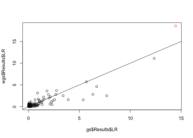
plot(x = gs$Results$LR, y = wgs$Results$LR, col = c('red', rep('black', 99)))
abline(a = 0, b = 1)
You can see that the weighted and unweighted version give similar results, but