netropy

netropy
You can install the released version of netropy from CRAN with:
install.packages("netropy")The development version from GitHub with:
# install.packages("devtools")
devtools::install_github("termehs/netropy")Multivariate entropy analysis is a general statistical method for analyzing and finding dependence structure in data consisting of repeated observations of variables with a common domain and with discrete finite range spaces. Only nominal scale is required for each variable, so only the size of the variable’s range space is important but not its actual values. Variables on ordinal or numerical scales, even continuous numerical scales, can be used, but they should be aggregated so that their ranges match the number of available repeated observations. By investigating the frequencies of occurrences of joint variable outcomes, complicated dependence structures, partial independence and conditional independence as well as redundancies and functional dependence can be found.
This package introduces these entropy tools in the context of network data. Brief description of various functions implemented in the package are given in the following but more details are provided in the package vignettes and the references listed.
library('netropy')The different entropy tools are explained and illustrated by exploring data from a network study of a corporate law firm, which has previously been analysed by several authors (link). The data set is included in the package as a list with objects representing adjacency matrices for each of the three networks advice (directed), friendship (directed) and co-work (undirected), together with a data frame comprising 8 attributes on each of the 71 lawyers.
To load the data, extract each object and assign the correct names to them:
data(lawdata)
adj.advice <- lawdata[[1]]
adj.friend <- lawdata[[2]]
adj.cowork <-lawdata[[3]]
df.att <- lawdata[[4]]A requirement for the applicability of these entropy tools is the specification of discrete variables with finite range spaces on the same domain: either node attributes/vertex variables, edges/dyad variables or triad variables. These can be either observed or transformed as shown in the following using the above example data set.
We have 8 vertex variables with 71 observations, two of which
(years and age) are numerical and needs
categorization based on their cumulative distributions. This
categorization is in details described in the vignette “variable domains
and data editing”. Here we just show the new dataframe created (note
that variable senior is omitted as it only comprises unique
values and that we edit all variable to start from 0):
att.var <-
  data.frame(
    status   = df.att$status-1,
    gender   = df.att$gender,
    office   = df.att$office-1,
    years    = ifelse(df.att$years <= 3,0,
                      ifelse(df.att$years <= 13,1,2)),
    age      = ifelse(df.att$age <= 35,0,
                      ifelse(df.att$age <= 45,1,2)),
    practice = df.att$practice,
    lawschool= df.att$lawschool-1
    )
head(att.var)
#>   status gender office years age practice lawschool
#> 1      0      1      0     2   2        1         0
#> 2      0      1      0     2   2        0         0
#> 3      0      1      1     1   2        1         0
#> 4      0      1      0     2   2        0         2
#> 5      0      1      1     2   2        1         1
#> 6      0      1      1     2   2        1         0
These vertex variables can be transformed into dyad variables by
using the function get_dyad_var(). Observed node attributes
in the dataframe att_var are then transformed into pairs of
individual attributes. For example, status with binary
outcomes is transformed into dyads having 4 possible outcomes \((0,0), (0,1), (1,0), (1,1)\):
dyad.status    <- get_dyad_var(att.var$status, type = 'att')
dyad.gender    <- get_dyad_var(att.var$gender, type = 'att')
dyad.office    <- get_dyad_var(att.var$office, type = 'att')
dyad.years     <- get_dyad_var(att.var$years, type = 'att')
dyad.age       <- get_dyad_var(att.var$age, type = 'att')
dyad.practice  <- get_dyad_var(att.var$practice, type = 'att')
dyad.lawschool <- get_dyad_var(att.var$lawschool, type = 'att')
Similarly, dyad variables can be created based on observed ties. For
the undirected edges, we use indicator variables read directly from the
adjacency matrix for the dyad in question, while for the directed ones
(advice and friendship) we have pairs of
indicators representing sending and receiving ties with 4 possible
outcomes :
dyad.cwk    <- get_dyad_var(adj.cowork, type = 'tie')
dyad.adv    <- get_dyad_var(adj.advice, type = 'tie')
dyad.frn    <- get_dyad_var(adj.friend, type = 'tie')
All 10 dyad variables are merged into one data frame for subsequent entropy analysis:
dyad.var <-
  data.frame(cbind(status   = dyad.status$var,
                  gender    = dyad.gender$var,
                  office    = dyad.office$var,
                  years     = dyad.years$var,
                  age       = dyad.age$var,
                  practice  = dyad.practice$var,
                  lawschool = dyad.lawschool$var,
                  cowork    = dyad.cwk$var,
                  advice    = dyad.adv$var,
                  friend    = dyad.frn$var)
                  )
head(dyad.var)
#>   status gender office years age practice lawschool cowork advice friend
#> 1      3      3      0     8   8        1         0      0      3      2
#> 2      3      3      3     5   8        3         0      0      0      0
#> 3      3      3      3     5   8        2         0      0      1      0
#> 4      3      3      0     8   8        1         6      0      1      2
#> 5      3      3      0     8   8        0         6      0      1      1
#> 6      3      3      1     7   8        1         6      0      1      1
A similar function get_triad_var() is implemented for
transforming vertex variables and different relation types into triad
variables. This is described in more detail in the vignette “variable
domains and data editing”.
The function entropy_bivar() computes the bivariate
entropies of all pairs of variables in the dataframe. The output is
given as an upper triangular matrix with cells giving the bivariate
entropies of row and column variables. The diagonal thus gives the
univariate entropies for each variable in the dataframe:
H2 <- entropy_bivar(dyad.var)
H2
#>           status gender office years   age practice lawschool cowork advice
#> status     1.493  2.868  3.640 3.370 3.912    3.453     4.363  2.092  2.687
#> gender        NA  1.547  3.758 3.939 4.274    3.506     4.439  2.158  2.785
#> office        NA     NA  2.239 4.828 4.901    4.154     5.058  2.792  3.388
#> years         NA     NA     NA 2.671 4.857    4.582     5.422  3.268  3.868
#> age           NA     NA     NA    NA 2.801    4.743     5.347  3.411  4.028
#> practice      NA     NA     NA    NA    NA    1.962     4.880  2.530  3.127
#> lawschool     NA     NA     NA    NA    NA       NA     2.953  3.567  4.186
#> cowork        NA     NA     NA    NA    NA       NA        NA  0.615  1.687
#> advice        NA     NA     NA    NA    NA       NA        NA     NA  1.248
#> friend        NA     NA     NA    NA    NA       NA        NA     NA     NA
#>           friend
#> status     2.324
#> gender     2.415
#> office     3.044
#> years      3.483
#> age        3.637
#> practice   2.831
#> lawschool  3.812
#> cowork     1.456
#> advice     1.953
#> friend     0.881
Bivariate entropies can be used to detect redundant variables that
should be omitted from the dataframe for further analysis. This occurs
when the univariate entropy for a variable is equal to the bivariate
entropies for pairs including that variable. As seen above, the
dataframe dyad.var has no redundant variables. This can
also be checked using the function redundancy() which
yields a binary matrix as output indicating which row and column
variables are hold the same information:
redundancy(dyad.var)
#> no redundant variables
#> NULL
More examples of using the function redundancy() is
given in the vignette “univariate bivariate and trivariate
entropies”.
Trivariate entropies can be computed using the function
entropy_trivar() which returns a dataframe with the first
three columns representing possible triples of variables
V1,V2, and V3 from the dataframe
in question, and their entropies H(V1,V2,V3) as the fourth
column. We illustrated this on the dataframe dyad.var:
H3 <- entropy_trivar(dyad.var)
head(H3, 10) # view first 10 rows of dataframe
#>        V1     V2        V3 H(V1,V2,V3)
#> 1  status gender    office       4.938
#> 2  status gender     years       4.609
#> 3  status gender       age       5.129
#> 4  status gender  practice       4.810
#> 5  status gender lawschool       5.664
#> 6  status gender    cowork       3.464
#> 7  status gender    advice       4.048
#> 8  status gender    friend       3.685
#> 9  status office     years       5.321
#> 10 status office       age       5.721
Joint entropies is a non-negative measure of association among pairs of variables. It is equal to 0 if and only if two variables are completely independent of each other.
The function joint_entropy() computes the joint
entropies between all pairs of variables in a given dataframe and
returns a list consisting of the upper triangular joint entropy matrix
(univariate entropies in the diagonal) and a dataframe giving the
frequency distributions of unique joint entropy values. A function
argument specifies the precision given in number of decimals for which
the frequency distribution of unique entropy values is created (default
is 3). Applying the function on the dataframe dyad.var with
two decimals:
J <- joint_entropy(dyad.var, 2)
J$matrix
#>           status gender office years  age practice lawschool cowork advice
#> status      1.49   0.17   0.09  0.79 0.38     0.00      0.08   0.02   0.05
#> gender        NA   1.55   0.03  0.28 0.07     0.00      0.06   0.00   0.01
#> office        NA     NA   2.24  0.08 0.14     0.05      0.13   0.06   0.10
#> years         NA     NA     NA  2.67 0.61     0.05      0.20   0.02   0.05
#> age           NA     NA     NA    NA 2.80     0.02      0.41   0.01   0.02
#> practice      NA     NA     NA    NA   NA     1.96      0.04   0.05   0.08
#> lawschool     NA     NA     NA    NA   NA       NA      2.95   0.00   0.01
#> cowork        NA     NA     NA    NA   NA       NA        NA   0.62   0.18
#> advice        NA     NA     NA    NA   NA       NA        NA     NA   1.25
#> friend        NA     NA     NA    NA   NA       NA        NA     NA     NA
#>           friend
#> status      0.05
#> gender      0.01
#> office      0.08
#> years       0.07
#> age         0.05
#> practice    0.01
#> lawschool   0.02
#> cowork      0.04
#> advice      0.18
#> friend      0.88
J$freq
#>       j  #(J = j) #(J >= j)
#> 1  0.79         1         1
#> 2  0.61         1         2
#> 3  0.41         1         3
#> 4  0.38         1         4
#> 5  0.28         1         5
#> 6   0.2         1         6
#> 7  0.18         2         8
#> 8  0.17         1         9
#> 9  0.14         1        10
#> 10 0.13         1        11
#> 11  0.1         1        12
#> 12 0.09         1        13
#> 13 0.08         4        17
#> 14 0.07         2        19
#> 15 0.06         2        21
#> 16 0.05         7        28
#> 17 0.04         2        30
#> 18 0.03         1        31
#> 19 0.02         5        36
#> 20 0.01         5        41
#> 21    0         4        45
As seen, the strongest association is between the variables
status and years with joint entropy values of
0.79. We have independence (joint entropy value of 0) between two pairs
of variables: (status,practice),
(practise,gender),
(cowork,gender),and
(cowork,lawschool).
These results can be illustrated in a association graph using the
function assoc_graph() which returns a ggraph
object in which nodes represent variables and links represent strength
of association (thicker links indicate stronger dependence). To use the
function we need to load the ggraph library and to
determine a threshold which the graph drawn is based on. We set it to
0.15 so that we only visualize the strongest associations
library(ggraph)
assoc_graph(dyad.var, 0.15)
Given this threshold, we see isolated and disconnected nodes
representing independent variables. We note strong dependence between
the three dyadic variables status,years and
age, but also a somewhat strong dependence among the three
variables lawschool, years and
age, and the three variables status,
years and gender. The association graph can
also be interpreted as a tendency for relations cowork and
friend to be independent conditionally on relation
advice, that is, any dependence between dyad variables
cowork and friend is explained by
advice.
A threshold that gives a graph with reasonably many small independent or conditionally independent subsets of variables can be considered to represent a multivariate model for further testing.
More details and examples of joint entropies and association graphs are given in the vignette “joint entropies and association graphs”.
The function prediction_power() computes prediction
power when pairs of variables in a given dataframe are used to predict a
third variable from the same dataframe. The variable to be predicted and
the dataframe in which this variable also is part of is given as input
arguments, and the output is an upper triangular matrix giving the
expected conditional entropies of pairs of row and column variables
(denoted \(X\) and \(Y\)) of the matrix, i.e. EH(Z|X,Y)
where \(Z\) is the variable to be
predicted. The diagonal gives EH(Z|X) , that is when only one
variable as a predictor. Note that NA’s are in the row and
column representing the variable being predicted.
Assume we are interested in predicting variable status
(that is whether a lawyer in the data set is an associate or partner).
This is done by running the following syntax
prediction_power('status', dyad.var)
#>           status gender office years   age practice lawschool cowork advice
#> status        NA     NA     NA    NA    NA       NA        NA     NA     NA
#> gender        NA  1.375  1.180 0.670 0.855    1.304     1.225  1.306  1.263
#> office        NA     NA  2.147 0.493 0.820    1.374     1.245  1.373  1.325
#> years         NA     NA     NA 2.265 0.573    0.682     0.554  0.691  0.667
#> age           NA     NA     NA    NA 1.877    1.089     0.958  1.087  1.052
#> practice      NA     NA     NA    NA    NA    2.446     1.388  1.459  1.410
#> lawschool     NA     NA     NA    NA    NA       NA     3.335  1.390  1.337
#> cowork        NA     NA     NA    NA    NA       NA        NA  2.419  1.400
#> advice        NA     NA     NA    NA    NA       NA        NA     NA  2.781
#> friend        NA     NA     NA    NA    NA       NA        NA     NA     NA
#>           friend
#> status        NA
#> gender     1.270
#> office     1.334
#> years      0.684
#> age        1.058
#> practice   1.427
#> lawschool  1.350
#> cowork     1.411
#> advice     1.407
#> friend     3.408
For better readability, the powers of different predictors can be
conveniently compared by using prediction plots that display a color
matrix with rows for \(X\) and columns
for \(Y\) with darker colors in the
cells when we have higher prediction power for \(Z\). This is shown for the prediction of
status:
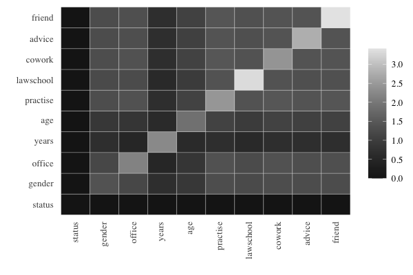
Obviously, the darkest color is obtained when the variable to be
predicted is included among the predictors, and the cells exhibit
prediction power for a single predictor on the diagonal and for two
predictors symmetrically outside the diagonal. Some findings are as
follows: good predictors for status are given by
years in combination with any other variable, and
age in combination with any other variable. The best sole
predictor is gender.
More details and examples of expected conditional entropies and prediction power are given in the vignette “prediction power based on expected conditional entropies”.
Occurring cliques in association graphs represent connected
components of dependent variables, and by comparing the graphs for
different thresholds, specific structural models of multivariate
dependence can be suggested and tested. The function
div_gof() allows such hypothesis tests for pairwise
independence of \(X\) and \(Y\): \(X \bot
Y\), and pairwise independence conditional a third variable \(Z\): \(X\bot
Y|Z\).
To test friend\(\bot\)
cowork\(|\)advice, that is whether
dyad variable friend is independent of cowork
given advice we use the function as shown below:
div_gof(dat = dyad.var, var1 = "friend", var2 = "cowork", var_cond = "advice")
#> the specified model of conditional independence cannot be rejected
#>      D df(D)
#> 1 0.94    12
Not specifying argument var_cond would instead test
friend\(\bot\)cowork without any
conditioning.
Parts of the theoretical background is provided in the package vignettes, but for more details, consult the following literature:
Frank, O., & Shafie, T. (2016). Multivariate entropy analysis of network data. Bulletin of Sociological Methodology/Bulletin de Méthodologie Sociologique, 129(1), 45-63. link