
![]()
![]()
An R package for identifying structural changes in time
series.
For modeling and forecasting time series it is essential to know whether the series are stationary or non-stationary since many commonly applied statistical methods (such as OLS) are invalid under non-stationarity. Two features that cause a time series to be non-stationary are considered here. On the one hand a time series can be subject to a change in mean, i.e. the expected value of the series changes over time. On the other hand a time series can be subject to a break in the autocovariance often refered to as a change in persistence, i.e. the dependence structure of the series changes over time.
The memochange package allows to consistently identify such changes in mean and persistence. This helps to avoid model misspecification and improve forecasting the series.
Potential examples for series with a change in mean and/or in persistence are found in the macroeconomic and financial area. This includes beta, inflation rates, interest rates, trading volume, volatilities, and so on.
You can install this R package from GitHub:
install.packages("devtools")
library(devtools)
install_github("KaiWenger/memochange")
or directly from the CRAN repository:
install.packages("memochange")In this section we present two short examples that illustrate how the implemented procedures can be used on a real data set. A more detailed presentation of the various tests and functions can be found in the vignettes.
As an empirical example for a time series that might exhibit a break
in persistence, we consider the price of crude oil. First, we download
the monthly price series from the FRED data base. For this purpose we
need the data.table package.
oil=data.table::fread("https://fred.stlouisfed.org/graph/fredgraph.csv?bgcolor=%23e1e9f0&chart_type=line&drp=0&fo=open%20sans&graph_bgcolor=%23ffffff&height=450&mode=fred&recession_bars=on&txtcolor=%23444444&ts=12&tts=12&width=1168&nt=0&thu=0&trc=0&show_legend=yes&show_axis_titles=yes&show_tooltip=yes&id=MCOILWTICO&scale=left&cosd=1986-01-01&coed=2019-08-01&line_color=%234572a7&link_values=false&line_style=solid&mark_type=none&mw=3&lw=2&ost=-99999&oet=99999&mma=0&fml=a&fq=Monthly&fam=avg&fgst=lin&fgsnd=2009-06-01&line_index=1&transformation=lin&vintage_date=2019-09-23&revision_date=2019-09-23&nd=1986-01-01")To get a first visual impression, we plot the series.
oil=as.data.frame(oil)
oil$DATE=zoo::as.Date(oil$DATE)
oil_xts=xts::xts(oil[,-1],order.by = oil$DATE)
zoo::plot.zoo(oil_xts,xlab="",ylab="Price",main="Crude Oil Price: West Texas Intermediate")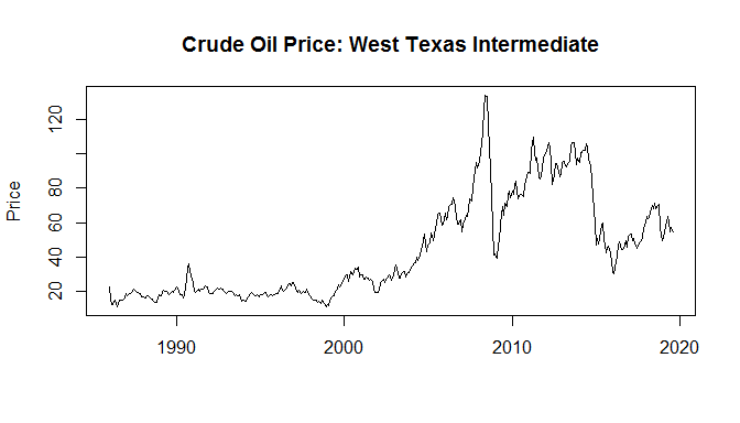
From the plot we observe that the series seems to be more variable in
its second part from year 2000 onwards. This is first evidence that a
change in persistence has occurred. We can test this hypothesis using
the functions cusum_test, LBI_test,
LKSN_test, MR_test, and
ratio_test. In this short example we only consider the MR
test as it is the most general one of the five implemented. The
functionality of the other tests is similar. They all require a
univariate numeric vector x as an input variable and yield
a matrix of test statistic and critical values as an output
variable.
library(memochange)
x <- as.numeric(oil[,2])
Applying the default version of the MR test by Martins and Rodrigues (2014) yields
MR_test(x)
#>                                          90%      95%      99% Teststatistic
#> Against increase in memory          4.270666 5.395201 8.233674      16.21494
#> Against decrease in memory          4.060476 5.087265 7.719128       2.14912
#> Against change in unknown direction 5.065695 6.217554 9.136441      16.21494
Here, test statistic and critical values for the null of constant persistence against an increase in persistence, a decrease in persistence, and a change in an unknown direction are displayed in a matrix. The latter accounts for the fact that we perform two tests facing a multiple testing problem. The results suggest that an increase in persistence has occurred somewhere in the series since the test statistic exceeds the critical value at the one percent level. In addition, this value is also significant when accounting for the multiple testing problem.
We can modify this default version by choosing the arguments
trend, tau, statistic,
serial, simu, and M. This amongst
other things allows the test to be also applied for series who are
suspected to exhibit linear trends or short run dynamics. Further
details can be found in the vignette and on the help page of the MR
test.
The test indicates that the oil price series exhibits an increase in
memory over time. To correctly model and forecast the series, the exact
location of the break is important. This can be estimated by the
BP_estim function. It is important for the function that
the direction of the change is correctly specified. In our case, an
increase in memory has occurred so that we set direction=“01”.
BP_estim(x,direction="01")
#> $Breakpoint
#> [1] 151
#>
#> $d_1
#> [1] 0.8127501
#>
#> $sd_1
#> [1] 0.08574929
#>
#> $d_2
#> [1] 1.088039
#>
#> $sd_2
#> [1] 0.07142857
This yields a list stating the location of the break (observation 151), semiparametric estimates of the order of integration (the persistence) in the two regimes (0.86 and 1.03) as well as the standard deviations of these estimates (0.13 and 0.15).
oil$DATE[151]
#> [1] "1998-07-01"
Consequently, the function indicates that there is a break in persistence in July, 1998. This means that from the beginning of the sample until June 1998 the series is integrated with an order of 0.85 and from July 1998 on the order of integration increased to 1.03.
The function further allows for various types of break point and persistence estimators. These are presented in the vignette.
As an empirical example for a persistent time series that might exhibit a change in mean, we consider the log squared returns of the NASDAQ in the time around the global financial crisis (2006-2009). First, we download the daily stock price series from the FRED data base.
nasdaq=data.table::fread("https://fred.stlouisfed.org/graph/fredgraph.csv?bgcolor=%23e1e9f0&chart_type=line&drp=0&fo=open%20sans&graph_bgcolor=%23ffffff&height=450&mode=fred&recession_bars=on&txtcolor=%23444444&ts=12&tts=12&width=1168&nt=0&thu=0&trc=0&show_legend=yes&show_axis_titles=yes&show_tooltip=yes&id=NASDAQCOM&scale=left&cosd=2006-01-01&coed=2009-01-01&line_color=%234572a7&link_values=false&line_style=solid&mark_type=none&mw=3&lw=2&ost=-99999&oet=99999&mma=0&fml=a&fq=Daily&fam=avg&fgst=lin&fgsnd=2009-06-01&line_index=1&transformation=lin&vintage_date=2019-11-04&revision_date=2019-11-04&nd=1971-02-05")We calculate the log squared returns as a measure of volatility and plot the series.
nasdaq              <- as.data.frame(nasdaq)
nasdaq[nasdaq=="."] <- NA
nasdaq              <- stats::na.omit(nasdaq)
nasdaq$NASDAQCOM    <- as.numeric(nasdaq$NASDAQCOM)
nasdaq$DATE=zoo::as.Date(nasdaq$DATE)
nasdaq_xts=xts::xts(nasdaq[,-1],order.by = nasdaq$DATE)
nasdaq_xts          <- log(diff(nasdaq_xts)^2)[-1]
zoo::plot.zoo(nasdaq_xts, xlab="", ylab="Log squared returns", main="Log squared returns of the NASDAQ")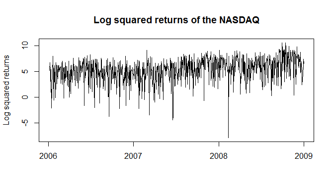
A first visual impression is that the mean seems to increase in the second part of the sample. Furthermore, applying the local Whittle estimator (choosing the bandwidth as T^0.65, which is usual in literature) we observe that there is the potential that the time series possess high persistence (d>0).
T           <- length(nasdaq_xts)
x           <- as.numeric(nasdaq_xts)
d_est       <- LongMemoryTS::local.W(x, m=floor(1+T^0.65))$d
round(d_est,3)
#> [1] 0.303
Therefore, to test whether a change in mean occured in the time
series one of the functions CUSUM_simple,
CUSUMfixed, CUSUMLM, fixbsupw,
snsupwald, snwilcoxon, and
wilcoxonLM have to be used. Here, we only consider a type
of the CUSUMfixed test since it contains the most user chosen arguments
among all seven implemented functions to test on a change in mean. The
functionality of the other tests is similar. All tests require a
univariate numeric vector x as an input variable and yield
a matrix of test statistic and critical values as an output
variable.
Applying the CUSUM fixed-m type A test of Wenger and Leschinski (2019)
with the previously estimated long-memory parameter and the recommended
bandwidth m=10 leads to
library(memochange)
CUSUMfixed(x,d=d_est,procedure="CUSUMfixedm_typeA",bandw=10)
#>           90%           95%           99% Teststatistic
#>         1.499         1.615         1.805         1.931
Here, test statistic and critical values for the null hypothesis of a constant mean against the alternative of a change in mean at some unknown point in time are displayed in a matrix. The results suggest that a change in mean has occurred somewhere in the series since the test statistic exceeds the critical value at the one percent level.
The test can be modified by choosing the arguments d,
procedure, bandw, and tau.
Depending on the kind of short run dynamics in the series, a different
bandwidth and/or procedure can be advantageous (see Wenger and
Leschinski (2019)). Further details can be found in the vignette and on
the help page of the CUSUMfixed test.
The test indicates that the log squared return series exhibits a
change in mean at some unknown point in time. To correctly model and
forecast the series, the exact location of the break is important. This
can be estimated by the breakpoints function from the
strucchange package.
BP       <- strucchange::breakpoints(x~1)$breakpoints
BP_index <- zoo::index(nasdaq_xts[BP])
BP_index
#> [1] "2007-07-23"
The function indicates that there is a break in persistence in July, 2007, which roughly corresponds to the start of the world financial crisis. The following plot shows the time series and the estimated means before and after the break
T_index  <- zoo::index(nasdaq_xts[T])
m1       <- mean(nasdaq_xts[1:BP])
m2       <- mean(nasdaq_xts[(BP+1):T])
zoo::plot.zoo(nasdaq_xts, xlab="", ylab="Log squared returns", main="Log squared returns of the NASDAQ")
graphics::segments(0,m1,BP_index,m1,col=2,lwd=2)
graphics::segments((BP_index+1),m2,T_index,m2,col=2,lwd=2)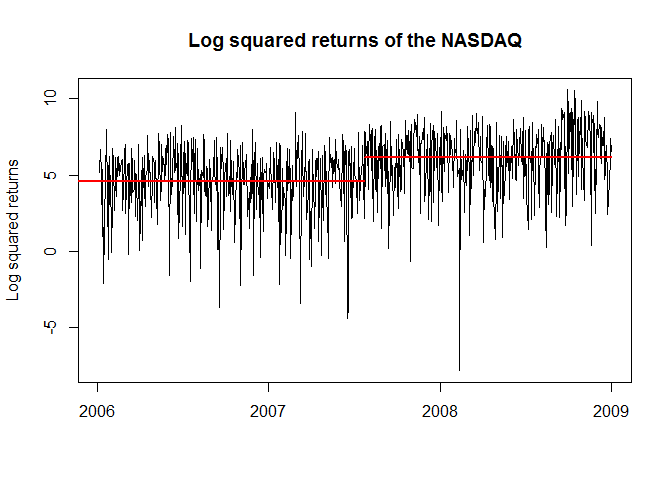
Martins, Luis F, and Paulo MM Rodrigues. 2014. “Testing for Persistence Change in Fractionally Integrated Models: An Application to World Inflation Rates.” Computational Statistics & Data Analysis 76: 502–22. https://doi.org/10.1016/j.csda.2012.07.021.
Wenger, Kai, and Christian Leschinski. 2019. “Fixed-Bandwidth Cusum Tests Under Long Memory.” Econometrics and Statistics. https://doi.org/10.1016/j.ecosta.2019.08.001.