![]()
![]()
The goal of forestploter is to create a
publication-ready forest plot with little effort. This package provides
some extra displays compared to other packages. The dataset will be used
as a basic layout for the forest plot. The width of the column to draw
the confidence interval can be controlled with the string length of the
column. Can use space to control this. The elements in the plot are put
in the rows and columns, think of the plot as a table.
You can install the development version of forestploter
from GitHub
with:
Install from CRAN
install.packages("forestploter")Install development version from GitHub
# install.packages("devtools")
devtools::install_github("adayim/forestploter")The column names of the provided data will be used as the header.
This is a basic example which shows you how to create a
forestplot:
library(grid)
library(forestploter)

dt <- read.csv(system.file("extdata", "example_data.csv", package = "forestploter"))

# Indent the subgroup if there is a number in the placebo column
dt$Subgroup <- ifelse(is.na(dt$Placebo),
                      dt$Subgroup,
                      paste0("   ", dt$Subgroup))

# NA to blank
dt$Treatment <- ifelse(is.na(dt$Treatment), "", dt$Treatment)
dt$Placebo <- ifelse(is.na(dt$Placebo), "", dt$Placebo)
dt$se <- (log(dt$hi) - log(dt$est))/1.96

# Add a blank column for the forest plot to display CI.
# Adjust the column width with space.
dt$` ` <- paste(rep(" ", 20), collapse = " ")

# Create confidence interval column to display
dt$`HR (95% CI)` <- ifelse(is.na(dt$se), "",
                             sprintf("%.2f (%.2f to %.2f)",
                                     dt$est, dt$low, dt$hi))

# Define theme
tm <- forest_theme(base_size = 10,
                   refline_col = "red",
                   arrow_type = "closed",
                   footnote_gp = gpar(col = "blue", cex = 0.6))

p <- forest(dt[,c(1:3, 20:21)],
            est = dt$est,
            lower = dt$low,
            upper = dt$hi,
            sizes = dt$se,
            ci_column = 4,
            ref_line = 1,
            arrow_lab = c("Placebo Better", "Treatment Better"),
            xlim = c(0, 4),
            ticks_at = c(0.5, 1, 2, 3),
            footnote = "This is the demo data. Please feel free to change\nanything you want.",
            theme = tm)

# Print plot
plot(p)
Sometimes one may want to change the color or font face of some
columns. Or one may want to insert text into certain rows. Or may want
an underline to separate by group. The function edit_plot,
add_text, insert_text, and
add_border can achieve these. Below is how to do this:
# Edit text in row 3
g <- edit_plot(p, row = 3, gp = gpar(col = "red", fontface = "italic"))

# Bold grouping text
g <- edit_plot(g,
               row = c(2, 5, 8, 11, 15, 18),
               gp = gpar(fontface = "bold"))

# Insert text at the top
g <- insert_text(g,
                 text = "Treatment group",
                 col = 2:3,
                 part = "header",
                 gp = gpar(fontface = "bold"))

# Add underline at the bottom of the header
g <- add_border(g, part = "header", row = 1, where = "top")
g <- add_border(g, part = "header", row = 2, where = "bottom")
g <- add_border(g, part = "header", row = 1, col = 2:3,
                gp = gpar(lwd = 2))

# Edit the background of row 5
g <- edit_plot(g, row = 5, which = "background",
               gp = gpar(fill = "darkolivegreen1"))

# Insert text
g <- insert_text(g,
                 text = "This is a long text. Age and gender summarised above.\nBMI is next",
                 row = 10,
                 just = "left",
                 gp = gpar(cex = 0.6, col = "green", fontface = "italic"))
g <- add_border(g, row = 10, col = 1:3, where = "top")
plot(g)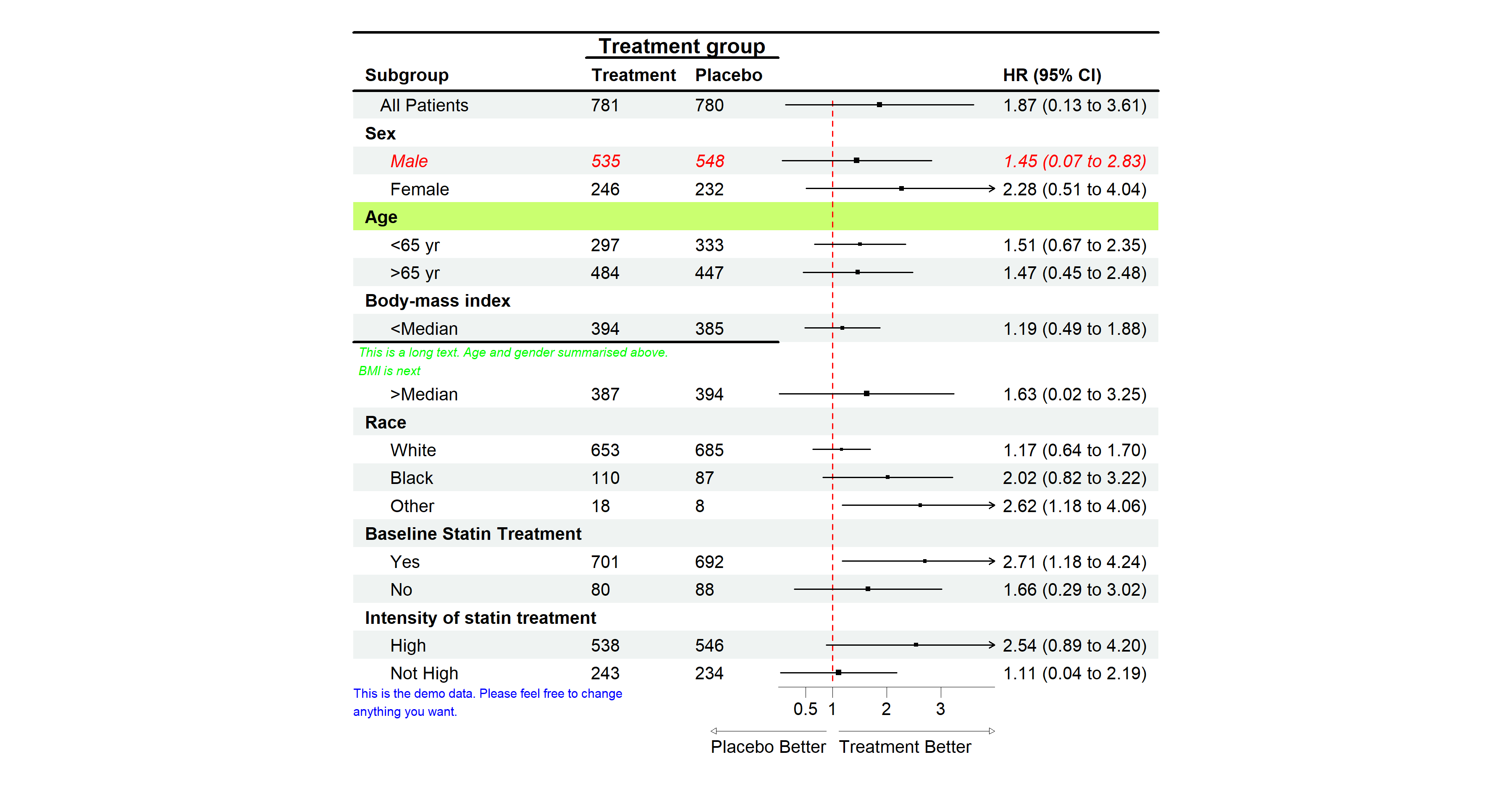
Remember to add 1 to the row number if you have inserted any text before. The row number will be changed after inserting a text.
If you want to draw CI to multiple columns, only need to provide a
vector of the position of the columns to be drawn in the data. As seen
in the example below, the CI will be drawn in columns 3 and 5. The first
and second est, lower, and upper
will be drawn in columns 3 and column 5.
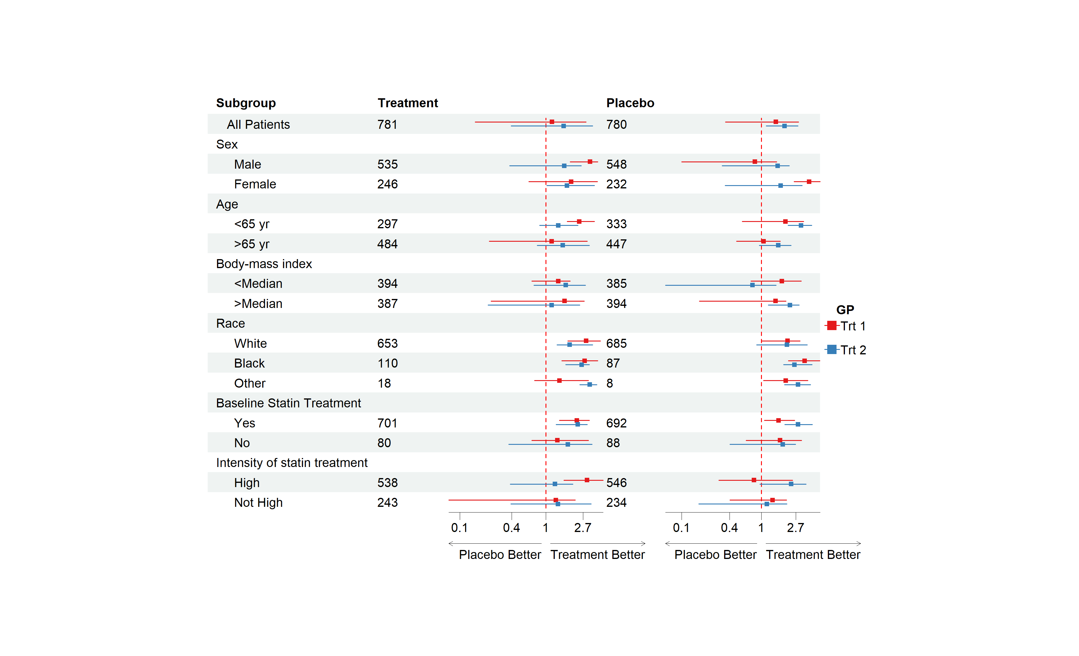
For a more complex example, you may want to draw CI by groups. The
solution is simple, just provide another set of est,
lower, and upper. If the number of provided
est, lower, and upper are larger
than the column number to draw CI, then the est,
lower, and upper will be reused. As it is
shown in the example below, est_gp1 and
est_gp2 will be drawn in column 3 and column 5 as normal.
But est_gp3 and est_gp4 haven’t been used,
those will be drawn to column 3 and column 5 again. So, the
est_gp1 and est_gp2 will be considered as
group 1, est_gp3 and est_gp4 group 2.
This is an example of multiple CI columns and groups:
# Add a blank column for the second CI column
dt$`   ` <- paste(rep(" ", 20), collapse = " ")

# Set-up theme
tm <- forest_theme(base_size = 10,
                   refline_col = "red",
                   footnote_gp = gpar(col = "blue"),
                   legend_name = "GP",
                   legend_value = c("Trt 1", "Trt 2"))

p <- forest(dt[,c(1:2, 20, 3, 22)],
            est = list(dt$est_gp1,
                       dt$est_gp2,
                       dt$est_gp3,
                       dt$est_gp4),
            lower = list(dt$low_gp1,
                         dt$low_gp2,
                         dt$low_gp3,
                         dt$low_gp4),
            upper = list(dt$hi_gp1,
                         dt$hi_gp2,
                         dt$hi_gp3,
                         dt$hi_gp4),
            ci_column = c(3, 5),
            ref_line = 1,
            arrow_lab = c("Placebo Better", "Treatment Better"),
            nudge_y = 0.2,
            x_trans = "log",
            theme = tm)

plot(p)