
The ‘chest’ package can be used to assess confounding effects by comparing effect estimates from many models. It calculates the changes in effect estimates by adding one of many variables (potential confounding factors) to the model sequentially in a stepwise fashion. Effect estimates can be regression coefficients, odds ratios and hazard ratios depending on the modelling methods. At each step, only one variable that causes the largest change in the effect estimates among the remaining variables is added to the model. Effect estimates and change (%) values are presented in a graph and data frame table. This approach can be used for assessing confounding effects in epidemiological studies and bio-medical research including clinical trials.
You can install the released version of chest from CRAN with:
install.packages("chest")A data frame ‘diab_df’ is used to examine the association between diabetes (Diabetes) and mortality (Endpoint). The purpose of using this data set is to demonstrate the use of the functions in this package rather than answering any research questions. Assuming it is a cohort design for Cox Proportional Hazards Models, cross-sectional design for Logistic Regression Model and matched cohort design for Conditional logistic regression Models.
‘chest_glm’ is slow. We can use ‘indicate = TRUE’ to monitor the progress.
chest_glm(crude = "Endpoint ~ Diabetes", xlist = vlist, data = diab_df, indicate = TRUE)
chest_cox(crude = "Surv(t0, t1, Endpoint) ~ Diabetes", xlist = vlist,
          na_omit = TRUE, data = diab_df, zero = 1)
#>       variables       HR       lb       ub     Change            p    n
#> 1         Crude 1.588134 1.434544 1.758167         NA 4.950249e-19 2048
#> 2         + CVD 1.526276 1.377192 1.691499 -3.8949795 7.454317e-16 2048
#> 3      + Income 1.480726 1.335380 1.641891 -2.9844079 9.581156e-14 2048
#> 4       + Smoke 1.514956 1.366037 1.680108  2.3116907 3.596810e-15 2048
#> 5         + Sex 1.498963 1.351879 1.662049 -1.0556582 1.571022e-14 2048
#> 6     + Married 1.512616 1.363974 1.677456  0.9108110 4.451213e-15 2048
#> 7         + Age 1.526426 1.376076 1.693202  0.9129952 1.305521e-15 2048
#> 8      + Cancer 1.517896 1.368399 1.683726 -0.5587865 3.050629e-15 2048
#> 9 + Education 1.514437 1.365204 1.679982 -0.2279234 4.453189e-15 2048chest_clogit(crude = "Endpoint ~ Diabetes + strata(mid)",
xlist = vlist, data = diab_df, indicate= TRUE, zero = 1)
#> 2 out of 9 3 out of 9 4 out of 9 5 out of 9 6 out of 9 7 out of 9 8 out of 9 9 out of 9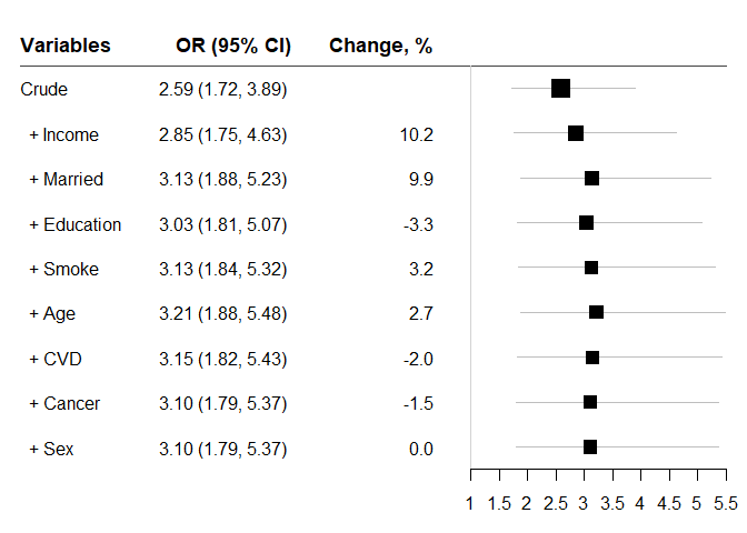
#>       variables       OR       lb       ub    Change            p    n
#> 1         Crude 2.586950 1.719871 3.891170        NA 5.033866e-06 2372
#> 2      + Income 2.850010 1.752942 4.633671 10.168718 2.405822e-05 2061
#> 3     + Married 3.133480 1.875838 5.234301  9.946296 1.283423e-05 2058
#> 4   + Education 3.030468 1.810620 5.072149 -3.287484 2.452619e-05 2048
#> 5       + Smoke 3.128331 1.839469 5.320260  3.229314 2.559384e-05 2048
#> 6         + Age 3.212487 1.883223 5.480007  2.690121 1.844153e-05 2048
#> 7         + CVD 3.148114 1.824571 5.431754 -2.003848 3.776568e-05 2048
#> 8      + Cancer 3.100427 1.790709 5.368067 -1.514782 5.340664e-05 2048
#> 9 + Sex 3.100427 1.790709 5.368067 0.000000 5.340664e-05 2048Because ‘chest’ fits many models and compares effect estimates, some analyses may take long time to complete.