![]()
![]()
![]()
The aim of the LMMsolver package is to provide an
efficient and flexible system to estimate variance components using
restricted maximum likelihood or REML (Patterson and Thompson 1971), for
models where the mixed model equations are sparse. An important feature
of the package is smoothing with P-splines (Eilers and Marx 1996). The
sparse mixed model P-splines formulation (Boer 2023) is used, which
makes the computations fast. The computational advantage of the sparse
mixed model formulation is especially clear for two-dimensional
smoothing (Boer 2023; Carollo et al. 2024).
install.packages("LMMsolver")remotes::install_github("Biometris/LMMsolver", ref = "develop", dependencies = TRUE)As an example of the functionality of the package we use the
USprecip data set in the spam package (Furrer
and Sain 2010).
library(LMMsolver)
library(ggplot2)

## Get precipitation data from spam
data(USprecip, package = "spam")

## Only use observed data.
USprecip <- as.data.frame(USprecip)
USprecip <- USprecip[USprecip$infill == 1, ]
head(USprecip[, c(1, 2, 4)], 3)
#>      lon   lat  anomaly
#> 6 -85.95 32.95 -0.84035
#> 7 -85.87 32.98 -0.65922
#> 9 -88.28 33.23 -0.28018
A two-dimensional P-spline can be defined with the
spl2D() function, with longitude and latitude as
covariates, and anomaly (standardized monthly total precipitation) as
response variable:
obj1 <- LMMsolve(fixed = anomaly ~ 1,
                 spline = ~spl2D(x1 = lon, x2 = lat, nseg = c(41, 41)),
                 data = USprecip)
The spatial trend for the precipitation can now be plotted on the map
of the USA, using the predict function of
LMMsolver:
lon_range <- range(USprecip$lon)
lat_range <- range(USprecip$lat)
newdat <- expand.grid(lon = seq(lon_range[1], lon_range[2], length = 200),
                      lat = seq(lat_range[1], lat_range[2], length = 300))
plotDat <- predict(obj1, newdata = newdat)

plotDat <- sf::st_as_sf(plotDat, coords = c("lon", "lat"))
usa <- sf::st_as_sf(maps::map("usa", regions = "main", plot = FALSE))
sf::st_crs(usa) <- sf::st_crs(plotDat)
intersection <- sf::st_intersects(plotDat, usa)
plotDat <- plotDat[!is.na(as.numeric(intersection)), ]

ggplot(usa) +
  geom_sf(color = NA) +
  geom_tile(data = plotDat,
            mapping = aes(geometry = geometry, fill = ypred),
            linewidth = 0,
            stat = "sf_coordinates") +
  scale_fill_gradientn(colors = topo.colors(100))+
  labs(title = "Precipitation (anomaly)",
       x = "Longitude", y = "Latitude") +
  coord_sf() +
  theme(panel.grid = element_blank())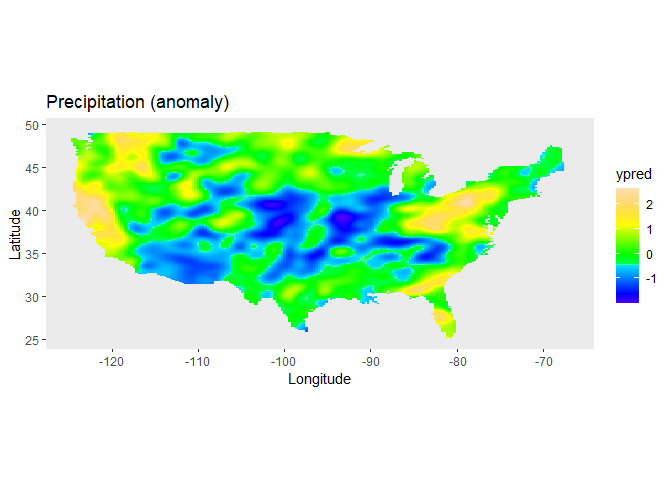
Further examples can be found in the vignette.
vignette("Solving_Linear_Mixed_Models")