D3 partition R is an R package to build interactive visualisation of nested data. Through easy to-use R functions (in a ggplot-like syntax) you will be able to plot and customise sunburst, treemap, circle treemap, icicle and partition chart. All the visualisations are interactive, zoom-able and based on the latest version of d3.js (V4).
The package is currently in beta and will soon be released on the CRAN. You can test it by installing the package from GitHub.
rmethods to add data library(devtools) install_github("AntoineGuillot2/D3partitionR")
The D3partitionR package uses a S3 class of object: D3partitionR objects. Two sets of methods are available, methods to add data (i.e. add_data, add_nodes_data, add_title) and methods to customise the chart (set_chart_type, set_labels_parameters, set_legend_parameter, …). These methods return a D3partitionR object which will be plotted and compiled by the plot method.
For this first example, we will use the Titanic data from Kaggle
## Loading packages
library("data.table")
library("D3partitionR")

## Reading data
titanic_data = fread("train.csv")

##Agregating data to have unique sequence for the 4 variables
var_names=c('Sex','Embarked','Pclass','Survived')
data_plot=titanic_data[,.N,by=var_names]
data_plot[,(var_names):=lapply(var_names,function(x){data_plot[[x]]=paste0(x,' ',data_plot[[x]])
  })]

## Plotting the chart
library("magrittr")
D3partitionR() %>%
  add_data(data_plot,count = 'N',steps=c('Sex','Embarked','Pclass','Survived')) %>%
  add_title('Titanic') %>%
  plot()
The add_data function is used to specify the data.frame to use and the variables to use:
You can easily change the type of chart with set_chart type.
##Treemap
D3partitionR() %>%
  add_data(data_plot,count = 'N',steps=c('Sex','Embarked','Pclass','Survived')) %>%
  set_chart_type('treemap') %>%
  plot()

##Circle treemap
D3partitionR() %>%
    add_data(data_plot,count = 'N',steps=c('Sex','Embarked','Pclass','Survived')) %>%
    set_chart_type('circle_treemap') %>%
plot()You can also add additional data for some nodes. For instance you can add comments on the nodes where the Embarking location is provided using the function add_nodes_data.
d3 = D3partitionR() %>%
  add_data(data_plot,count = 'N',tooltip=c('name','Location'),steps=c('Sex','Embarked','Pclass','Survived')) %>%
  add_nodes_data(list('Embarked S'=list('Location'='<a href="https://fr.wikipedia.org/wiki/Southampton">Southampton</a>'),
                 'Embarked C'=list('Location'='<a href="https://fr.wikipedia.org/wiki/Cherbourg-Octeville">Cherbourg</a>'),
                 'Embarked Q'=list('Location'='<a href="https://fr.wikipedia.org/wiki/Cobh">Queenstown</a>')
                 )
                 )
d3 %>%
  set_legend_parameters(zoom_subset = TRUE) %>%
  set_chart_type('circle_treemap') %>%
  set_tooltip_parameters(visible=TRUE, style='background-color:lightblue;',builder='basic') %>%
  plot()
With this code, the nodes Embarked S, Embarked C, Embarked Q will
have additional data apended (the url of the wikipedia page of the
location). 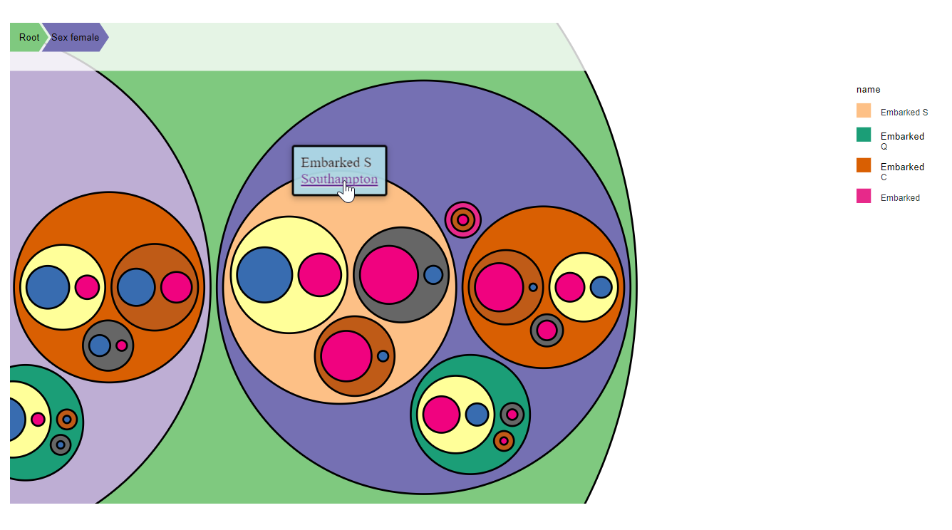
The add_data also contains parameters to specify the variables to used as:
D3partitionR() %>%
  add_data(data_plot,count = 'N',steps=c('Sex','Embarked','Pclass','Survived'),tooltip=c('name','N'),label='name',color='N') %>%
  set_chart_type('treemap') %>%
  plot()
These variables should either be:
titanic_data = fread("train.csv")

## Selecting variables
var_names = c('Sex','Embarked','Pclass','Survived')

## Merging steps data and data with ages
data_plot = merge(titanic_data[,.N, by = c(var_names)], titanic_data[,.(mean_age=mean(Age,na.rm =TRUE), Survived_num=Survived), by=c(var_names)], by=var_names)

##Improving steps naming
data_plot[,(var_names):=lapply(var_names,function(x){data_plot[[x]]=paste0(x,' ',data_plot[[x]])
  })]

D3partitionR()%>%
  add_data(data_plot,count = 'N',steps=c('Sex','Embarked','Pclass','Survived'),tooltip=c('name','N','mean_age'),label='name',color='Survived_num',aggregate_fun = list(mean_age=weighted.mean,Survived_num=weighted.mean)) %>%
  set_chart_type('treemap') %>%
  set_labels_parameters(cut_off=10) %>%
  plot()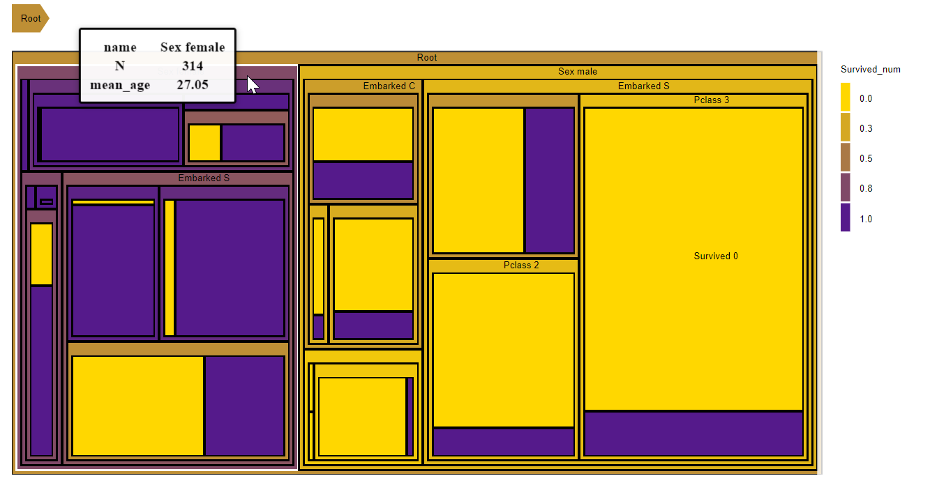
The modification of legend, labels and tooltips parameters are easily done too.
To modify the legend parameters, you need to use set_legend_parameters, it has three parameters.
##Circle treemap
D3partitionR()%>%
    add_data(data_plot,count = 'N',steps=c('Sex','Embarked','Pclass','Survived'))%>%
    set_legend_parameters(visible=T,zoom_subset=T,width=100)%>%
    plot()
The use of visible and width are obvious. On the other hand, the zoom_subset will enable or disable the filtering of the legend labels based on the current level of zoom. If the zoom_subset is set to TRUE, only the direct children of the current root are shown in the legend.
To modify the tooltips parameters, you need to use set_tooltip_parameters, it has three parameters.
##Circle treemap
D3partitionR()%>%
    add_data(data_plot,count = 'N',steps=c('Sex','Embarked','Pclass','Survived'))%>%
    set_tooltip_parameters(visible=T,style='background-color:lightblue;',builder='basic')%>%
    plot()
The style argument is used to customise the tooltips using a CSS string. The builder parameter changes the type of tooltip using a js expression. Two builders are currently in the package (‘basic’ and ‘table’).
To modify the labels parameters, you need to use set_tooltip_parameters, it has three parameters.
##Circle treemap
D3partitionR()%>%
    add_data(data_plot,count = 'N',steps=c('Sex','Embarked','Pclass','Survived'))%>%
    set_label_parameters(visible=T,cut_off=3,style='fill:lightblue;')%>%
    plot()
The style argument is used to customise the labels using a CSS string. The cut_off parameter is used to choose which proportion of the labels is to be shown. For instance if the cut-off is set to 3, only the labels belonging to a node with a size which is greater than 3% of the current root size will be displaued.
The trail can only be enabled/disabled using set_trail
A title can be added using add_title which has two parameters text to provide the text and style.
##Circle treemap
D3partitionR()%>%
    add_data(data_plot,count = 'N',steps=c('Sex','Embarked','Pclass','Survived'))%>%
    add_title(text='Titanic',style='font-size:20px;')%>%
plot()The d3.js code was thought to be modular, hence it is easy to add new chart types. Each chart type has its own .js file with its drawing function. In this file:
Hence any hierarchical-like d3.js visualisation can easily be generalised and added to the package