 ======================================================================================================

[](https://travis-ci.com/Jean-Romain/lidR)
[](https://codecov.io/gh/Jean-Romain/lidR?branch=master)
R package for Airborne LiDAR Data Manipulation and Visualization for Forestry Applications
The lidR package provides functions to read and write `.las` and `.laz` files, plot point clouds, compute metrics using an area-based approach, compute digital canopy models, thin lidar data, manage a catalog of datasets, automatically extract ground inventories, process a set of tiles using multicore processing, individual tree segmentation, classify data from geographic data, and provides other tools to manipulate LiDAR data in a research and development context.
* Development of the `lidR` package between 2015 and 2018 was made possible thanks to the financial support of the [AWARE project (NSERC CRDPJ 462973-14)](http://aware.forestry.ubc.ca/); grantee [Prof Nicholas Coops](http://profiles.forestry.ubc.ca/person/nicholas-coops/).
* Development of the `lidR` package between 2018 and 2019 was made possible thanks to the financial support of the Ministère des Forêts, de la Faune et des Parcs of Québec.
:book: Read the [Wiki pages](https://github.com/Jean-Romain/lidR/wiki) to get started with the lidR package.
# Key features
======================================================================================================

[](https://travis-ci.com/Jean-Romain/lidR)
[](https://codecov.io/gh/Jean-Romain/lidR?branch=master)
R package for Airborne LiDAR Data Manipulation and Visualization for Forestry Applications
The lidR package provides functions to read and write `.las` and `.laz` files, plot point clouds, compute metrics using an area-based approach, compute digital canopy models, thin lidar data, manage a catalog of datasets, automatically extract ground inventories, process a set of tiles using multicore processing, individual tree segmentation, classify data from geographic data, and provides other tools to manipulate LiDAR data in a research and development context.
* Development of the `lidR` package between 2015 and 2018 was made possible thanks to the financial support of the [AWARE project (NSERC CRDPJ 462973-14)](http://aware.forestry.ubc.ca/); grantee [Prof Nicholas Coops](http://profiles.forestry.ubc.ca/person/nicholas-coops/).
* Development of the `lidR` package between 2018 and 2019 was made possible thanks to the financial support of the Ministère des Forêts, de la Faune et des Parcs of Québec.
:book: Read the [Wiki pages](https://github.com/Jean-Romain/lidR/wiki) to get started with the lidR package.
# Key features
 ### Read and display a las file
In R-fashion style the function `plot`, based on `rgl`, enables the user to display, rotate and zoom a point cloud. Because `rgl` has limited capabilities with respect to large datasets, we also made a package [PointCloudViewer](https://github.com/Jean-Romain/PointCloudViewer) with greater display capabilities.
```r
las <- readLAS("
### Read and display a las file
In R-fashion style the function `plot`, based on `rgl`, enables the user to display, rotate and zoom a point cloud. Because `rgl` has limited capabilities with respect to large datasets, we also made a package [PointCloudViewer](https://github.com/Jean-Romain/PointCloudViewer) with greater display capabilities.
```r
las <- readLAS("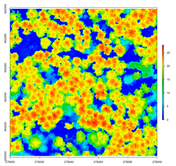 `lidR` has several algorithms from the literature to compute canopy height models either point-to-raster based or triangulation based. This allows testing and comparison of some methods that rely on a CHM, such as individual tree segmentation or the computation of a canopy roughness index.
```r
las <- readLAS("
`lidR` has several algorithms from the literature to compute canopy height models either point-to-raster based or triangulation based. This allows testing and comparison of some methods that rely on a CHM, such as individual tree segmentation or the computation of a canopy roughness index.
```r
las <- readLAS(" `lidR` enables the user to manage, use and process a catalog of `las` files. The function `catalog` builds a `LAScatalog` object from a folder. The function `plot` displays this catalog on an interactive map using the `mapview` package (if installed).
```r
ctg <- catalog("
`lidR` enables the user to manage, use and process a catalog of `las` files. The function `catalog` builds a `LAScatalog` object from a folder. The function `plot` displays this catalog on an interactive map using the `mapview` package (if installed).
```r
ctg <- catalog(" The `lastrees` function has several algorithms from the literature for individual tree segmentation, based either on the digital canopy model or on the point-cloud. Each algorithm has been coded from the source article to be as close as possible to what was written in the peer-reviewed papers. Our goal is to make published algorithms usable, testable and comparable.
```r
las <- readLAS("
The `lastrees` function has several algorithms from the literature for individual tree segmentation, based either on the digital canopy model or on the point-cloud. Each algorithm has been coded from the source article to be as close as possible to what was written in the peer-reviewed papers. Our goal is to make published algorithms usable, testable and comparable.
```r
las <- readLAS(" Most of the lidR functions can process seamlessly a set of tiles and return a continuous output. Users can create their own methods using the LAScatalog processing engine via the `catalog_apply` function. Among other features the engine takes advantage of point indexation with lax files, takes care of processing tiles with a buffer and allows for processing big files that do not fit in memory.
```r
# Load a LAScatalog instead of a LAS file
ctg <- catalog("
Most of the lidR functions can process seamlessly a set of tiles and return a continuous output. Users can create their own methods using the LAScatalog processing engine via the `catalog_apply` function. Among other features the engine takes advantage of point indexation with lax files, takes care of processing tiles with a buffer and allows for processing big files that do not fit in memory.
```r
# Load a LAScatalog instead of a LAS file
ctg <- catalog("LAScatalog processing engine
- Overview
- High level API
- Control of the chunk size
- Control of the chunk buffer
- Control of the chunk alignment
- Filter points
- Select attributes
- Write independent chunks on disk
- Modification of the file format
- Progress estimation
- Error handling
- Empty chunks
- Parallel processing
- Overlapping tiles
- Partial processing
- Partial output
- Low level API
- Advanced usages of the engine
In lidR the LAScatalog processing engine refers to the function catalog_apply(). This function is the core of the package and drives, internally, every single other function that is capable of processing a LAScatalog including clip_roi(), find_trees(), grid_terrain(), decimate_points() and many others as well as some experimental functions in third party packages such as lidRplugins. This engine is powerful and versatile but also relatively hard to understand for new users and especially for R beginners. This vignettes documents how it works going deeper and deeper inside the engine. It is highly recommended to read the vignette named LAScatalog formal class before to enter this one even if one may find some overlap between these two vignettes.
Overview
When processing a LAScatalog the area covered is split into chunks. A chunk can be seen as a square region of interest (ROI) and all together the chunks cover the collection of file. The collection of files is not physically split, the chunks correspond to a virtual splitting of the coverage. Then the chunk are processed sequentially (one after the other) or in parallel but always independently. To process each chunk, the corresponding point-cloud is extracted from the collection of files and loaded into memory. Any function can be applied on these independent point-clouds and the independent outputs are stored in a list. The list contains one output per chunk and once each chunk is processed the list is collapsed into a single continuous valid object such as a RasterLayer or a SpatialPolygonsDataFrame. The roles of the catalog engine are to:
- Create a set of chunk that encompass the collection of files
- Load a buffer on-the-fly around each chunk
- Apply any user-defined function on the loaded point clouds
- Take care of parallelism by computing several chunks at a time sending computation on multiple cores or even on multiple machines
- Take care of error handling including the management of logs in case of crash and the capability to return a partial output in case of crash at mid-computation
- Provide a visual monitoring of the computation progress in real time including a feedback on successes, warnings and errors.
- Merge the independent outputs into a single continuous object.
When using the LAScatalog engine, users only need to think about what function they want to apply over their coverage, all the above mentioned features being managed internally. There are many possible processing tuning and this is why one may feel lost by all the options to consider. To simplify we can make two categories of tools:
- High level API are
lidRfunctions that perform a given operation either on aLASorLAScatalogobject transparently in a straightforward way. For examplesgrid_metrics(),grid_terrain(),find_trees()are high level API. Rule of thumbs, if the functioncatalog_apply()is not directly used it is high level API. Processing options can be tuned with functions that start byopt_(for option). - Low level API is the function
catalog_apply()itself. This function is designed to build new high level applications and is used internally by all thelidRfunctions but can also be used by users to build their own tools. Options can be tuned with the parameter.optionsofcatalog_apply().
In the following vignette we will discuss first of the hight level API then of the low level API. The variables named ctg* will refer to a LAScatalog object in subsequent codes.
High level API
Control of the chunk size
The catalog takes care of making chunks and user can define the size of the chunks. By default this size is set to 0 meaning that a chunk is a file and thus each files will be processed sequentially. The chunk size is not the most important option. It is mainly intended to be used with small configuration computers to do not load too many points at once. Reducing or increasing the chunk size does not modify the output but it reduces the memory used by reducing the quantity of points loaded. It is recommended to set this options to 0 but sometime it is a good idea to set a small size to process particularly big files.
opt_chunk_size(ctg) <- 0 # Processing by files
plot(ctg, chunk = TRUE)
opt_chunk_size(ctg) <- 900 # Processing chunks of 900 x 900
plot(ctg, chunk = TRUE)

Control of the chunk buffer
Each chunk is loaded with a buffer around it to ensure that independent clouds will not be affected by edge effects. For example when computing a digital terrain model if a buffer is not loaded, the terrain is weakly computed at the edge of the point cloud because of the absence of context in the neighbourhood. The chunk buffer size is the most important option. A too small buffer can create incorrect outputs. The default is 30 m and is likely to be appropriated for most use cases.
opt_chunk_buffer(ctg) <- 0 # No buffer
plot(ctg, chunk = TRUE)
opt_chunk_buffer(ctg) <- 200 # 200 m buffer
plot(ctg, chunk = TRUE)
lidR functions always checks if an appropriate buffer is set. For example it is impossible to apply grid_terrain() with no buffer.
Control of the chunk alignment
In some cases it might be suitable to control the alignment of the chunks to force a given pattern. This is a rare use case but the engine supports such possibility. This option is obviously meaningless when processing by file. The chunk alignment is not the most important option and does not modify the output but it may generate more or less chunks depending on the alignment. However it might be very useful is the particular case of the function catalog_retile() for example to control accurately the new tiling pattern.
opt_chunk_size(ctg) <- 2000
opt_chunk_buffer(ctg) <- 0
plot(ctg, chunk = TRUE)
opt_chunk_size(ctg) <- 2000
opt_chunk_buffer(ctg) <- 0
opt_chunk_alignment(ctg) <- c(1000, 1000)
plot(ctg, chunk = TRUE)

clip_roi() is the single case where the control of the chunk is not respected. clip_roi() aims to extract a shape (rectangle, disc, polygon) as a single entity . The chunk pattern does not make sense here.
Filter points
When reading a single file with readLAS() the option filter allows for discarding some points based on criteria. For example -keep_first keeps only first returns and discard all non first returns. It is important to understand that the discarded points are discarded while reading and they will never be loaded in memory. This is useful to process only some points of interest for example when computing metrics only on first returns above 2 m.
# Read all the points
readLAS("file.las")
# Only first returns above 2 m are loaded
readLAS("file.las", filter = "-drop_first -drop_z_below 2")This works only when the readLAS() function is called explicitly. When using the catalog processing engine, readLAS() is called internally under the hood and users cannot explicitly call the filter argument. filter is propagated with the opt_filter() function.
Internally, for each chunk, readLAS() will be called with filter = "-drop_first -drop_z_below 2 in every functions that is processing a LAScatalog unless the documentation explicitly mention something else. In the following examples clip_roi() is used to extract a plot but only the points classified as ground or water will be read and grid_metrics() is used to compute metrics only on first returns above 2 meters. It does not mean other points do not exist, they are simply not read.
opt_filter(ctg) <- "-keep_class 2 9"
las <- clip_disc(ctg, 273400, 5274500, 20)
opt_filter(ctg) <- "-keep_first -drop_z_below 2"
m <- grid_metrics(ctg, .stdmetrics, 20)All filters are not necessarily appropriated everywhere. For example the following is meaningless because it discards all the point that are used to compute a DTM.
Select attributes
When reading a single file with readLAS() the option select allows for discarding some attributes of the points. For example select = "ir" keeps only the intensity and the return number of each point and discards all the other attributes such as the scan angle, the flags or the classification. Its role is only to save processing memory by do not loading data that are not actually needed. Similarly to opt_filter() the function opt_select() allows to propagate the argument select to readLAS().
# Load Intensity only
opt_select(ctg) <- "i"
las <- clip_disc(ctg, 273500, 5274500, 10)
# Load Intensity + Classification + ReturnNumber + NumberOfReturns
opt_select(ctg) <- "icrn"
las <- clip_disc(ctg, 273500, 5274500, 10)However this option is not always respected because many lidR functions already know which optimization they should apply. In the following example the ‘classification’ attribute is explicitly discarded but yet the creation of a DTM do works because the function overwrites the user settings for something better (in this specific case xyzc).
Write independent chunks on disk
By default every function returns a continuous output within a single R object stored in memory so it is immediately usable in the working environment in a straightforward way. For example a SpatialPointsDataFrame for find_trees().
# Find the trees
trees <- find_trees(ctg2, lmf(3))
# The trees are immediately usable in subsequent analysis
trees
#> class : SpatialPointsDataFrame
#> features : 292
#> extent : 481260, 481349.9, 3812921, 3813011 (xmin, xmax, ymin, ymax)
#> crs : +proj=utm +zone=12 +datum=NAD83 +units=m +no_defs +ellps=GRS80 +towgs84=0,0,0
#> variables : 2
#> names : treeID, Z
#> min values : 1, 2.16
#> max values : 292, 32.07However in some case this behaviour might not be suitable especially for big collection of files that cover a broad area. In this case the computer will maybe not be able to handle so much data and/or will run into trouble when merging the different independent chunks into a single object. This is why the engine has the capability to write on disk the output of each independent chunks. The function opt_output_files() can be used to set a path on disk where the output of each chunk should be saved on disk. This path is templated so the engine is able to create a different file name for each chunk. The general form is the following:
The templates can be XCENTER, YCENTER, XLEFT, YBOTTOM, XRIGHT, YTOP, ID or ORIGINALFILENAME. The templated string does not contain the file extension. The engine guesses the extension and it works no matter the output. For example:
# Force the results to be written on disk
opt_output_files(ctg2) <- paste0(tempdir(), "/tree_coordinate_{XLEFT}_{YBOTTOM}")
trees <- find_trees(ctg2, lmf(3))
# The output has been modified by this options and it now gives
# the paths to the written files (here shapefiles)
trees
#> [1] "/tmp/RtmpU5qnB2/tree_coordinate_481250_3812750.shp"
#> [2] "/tmp/RtmpU5qnB2/tree_coordinate_481250_3813000.shp"The is one file per chunk and thus processing by file with the template {ORIGINALFILENAME} or its shortcut {*} may be suitable to further match the output files with the point cloud files. However depending on the size of the file and the capacity of the computer it is not always possible (see section “Control of the chunk size”).
In the previous example, several shapefiles were written on disk and there is no way to combine them into a single light R object. But sometime it is possible to return a light object that aggregates all the written files. For rasters for example it is possible to build a virtual raster mosaic. The engine automatically do that when it is possible.
# Force the results to be written on disk
opt_output_files(ctg2) <- paste0(tempdir(), "/tree_coordinate_{XLEFT}_{YBOTTOM}")
chm <- grid_canopy(ctg2, 1, p2r())
# Many raster have been written on disk
# but a light RasterLayer has been returned anyway
chm
#> class : RasterLayer
#> dimensions : 90, 90, 8100 (nrow, ncol, ncell)
#> resolution : 1, 1 (x, y)
#> extent : 481260, 481350, 3812921, 3813011 (xmin, xmax, ymin, ymax)
#> crs : +proj=utm +zone=12 +ellps=GRS80 +towgs84=0,0,0,0,0,0,0 +units=m +no_defs
#> source : /tmp/RtmpU5qnB2/grid_canopy.vrt
#> names : layer
#> values : 0, 32.07 (min, max)There are two special cases. The first one is when raster files are written. They are merged into a valid RasterLayer using a virtual mosaic. The second one is when LAS or LAZ files are written on disk. They are merged into a LAScatalog.
opt_output_files(ctg2) <- "{tempdir()}/plot_{ID}"
new_ctg <- clip_disc(ctg2, x, y, 20)
plot(ctg2)
points(x,y)
plot(new_ctg)

Modification of the file format
By default, rasters are written in GeoTiff files, spatial points, spatial polygons and spatial lines either in sp or sf formats are written in ESRI shapefiles, point-clouds are written in las files and table are written in csv files. This can be modified at any time by users but it corresponds to advanced settings and thus this section is deferred in a later section about advanced usages. However the function opt_laz_compression() is a simple shortcut to switch from las to laz when writing a point cloud.
Progress estimation
The engine provides a real time display of the progression that serves two purposes: (a) see the progression and (b) monitor troubleshooting. It is enabled by default and when a LAScatalog is processing a chart is displayed. The chunks are progressively coloured. No colour, the chunk is pending. Blue, the chunk is processing. Green, the chunk has been processed. Orange, the chunk has been processed with a warning. Red, the chunk processing failed.

This can be disabled with:
Error handling
If a chunks produced a warning this is rendered in real time with an orange colouring. However the message(s) of the warning(s) are delayed and printed only at the end of the computation.

If a chunks produced an error this is rendered in real time as well. The computation stops as usual but the error is handle in such a way that the code did not actually failed. The functions returned a partial output i.e. the output of the tiles that were computed successfully. A message is printed telling user where and what was the error and suggest to load this specific section of the catalog to test what was wrong with it. In the following case one tile was not classified so it failed.
#> An error occurred when processing the chunk 30. Try to load this chunk with:
#> chunk <- readRDS("/tmp/RtmpTozKLu/chunk30.rds")
#> las <- readLAS(chunk)
#> No ground point found.
The engine logged the chunk and it is easy to load this specific processing region for further investigation by copy pasting the mentioned code.
The engine is able to bypass the error. This can be activated with opt_stop_early() and the computation will run till the end in any case. In this case chunks that failed will be missing and the output will contain holes with missing data. We do not recommend the use of such option because other errors will be bypassed as well without triggering any informative message. This option exists and can be useful if used carefully. Users should always try to fix the problem.

Empty chunks
Sometime some chunks are empty and we discover that only when loading the region of interest. This may happens when the chunk pattern is different from the tiling pattern because some chunks may have been created but they do not actually encompass any point. This is the case when the file is only partially populated because the bounding box of the file/tile is bigger than its actual content. This often happens on the edge of the collection. In this case the engine displays the chunks in gray. This may also happens if filter is set in such a way that a lot of points are discarded and in some chunks all the points appear to be discarded. Those chunk are displayed in gray.

Parallel processing
The engine takes care of processing the chunks one after the other sequentially or in parallel. The parallelisation can be done with a single machine or on multiple machines by sending the chunks to different workers. The parallelization is performed using the framework given by the package future. Understanding the basic of this package is thus required. To activate a paralellization strategy users need to register a strategy with future. For example:
Now 4 chunks will be processed at a time and the engine monitoring displays in real time the processing chunks:

However parallel processing is not magic. First of all it loads several point clouds at one time because several chunks are read at one time. Users must ensure they have enough RAM to support that. Second, there are strong overheads at parallelizing tasks. Putting all cores on a task does not always make it faster!
Overlapping tiles
In lidR if some files are overlapping each other, a message is printing to alert about potential troubles.
ctg <- readLAScatalog("path/to/folder/")
#> Be careful, some tiles seem to overlap each other. lidR may return incorrect outputs with edge artifacts when processing this catalog.Overlapping is not an issue by itself. The actual problem is duplicated points. Because lidR makes arbitrary chunks, users are likely to load twice the same points is some areas are duplicated in the original dataset. Below few classical cases of overlapping files:
The files are already buffered: the engine is designed to work with a continuous dataset. If files are already buffered users have several options to process the collection but they all imply to drive without security belt. The first and best option is to skip the buffer at read time assuming that buffer points are flagged somehow. For example flagged as withheld:
If it is not the case one can try to retile the
LAScatalogwith a negative buffer to remove the buffer.opt_chunk_size(ctg) <- 0 opt_output_files(ctg) <- "/data/unbufferd/{ORIGINALFILENAME}" opt_chunk_buffer(ctg) <- -40 new_ctg <- catalog_retile(ctg)It is also possible to process by file without buffer by disabling all the internal controls using
opt_wall_to_wall(). Using this disables the guarantee of having a correct, valid, continuous result. This is a free wheel mode.- The files are flight-lines: when a file records a single flight transect, files are overlapping, of course, but this does not create regions with duplicated points. You can process normally and ignore the message. The engine will take care of making independent and buffered chunks.
- There are some duplicated files: a few tiles that appear more than once. When plotting the
LAScatalog, the light blue being transparent, the overlapping regions should appears darker. You must remove these files. Other: there are certainly many other reasons to get overlaps.
Partial processing
It is possible to process only a subregion of the collection by flagging some files. In this case only the flagged files will be process but the neighbouring tiles are used to load a buffer so the local context is not lost. Below only 4 files are flagged and the display plots the other tiles almost white.

Partial output
As mentioned in a previous section when an error stops the computation the output is never NULL it contains a valid output computed from the part of the catalog that have been processed. It is a partial but valid output. Hopefully next versions of the package will allow to restart a computation that failed from the failing points
Low level API
The low level API refers to the use of catalog_apply(). This function drives every single other one and is intended to be used by developers to create new processing routines that are not existing in lidR. When catalog_apply() is running it respects all the processing option we have seen so far plus some developer’s constraints that are not intended to be modified by users. catalog_apply() maps any R function but such function must respect some rules.
Making a valid function for catalog_apply()
A function mapped by catalog_apply() must take a chunk as input and must read the chunk using readLAS(). So a valid function starts like that:
The size of the chunks, the size of the buffer and the positioning of the chunks depend on the option carried by the LAScatalog and set with opt_chunk_*() functions. In addition the select and filter argument cannot be specified in readLAS(). They are controlled by opt_filter() and opt_select() as seen in previous sections. The problem with that is that if any size of chunk can be defined it is possible to create chunks that encompass a tile but that do not contain any points. So sometime readLAS(chunk) may return a point cloud with 0 point (see section ‘empty chunks’). In that case subsequent code is likely to fail. As a consequence the function mapped by catalog_apply() must check for empty chunks and return NULL. When returning NULL the engine understand that the chunk was empty.
The following code does not work because catalog_apply() checks internally if the function returns NULL for empty chunks
routine <- function(chunk){
las <- readLAS(chunk)
}
catalog_apply(ctg, routine)
#> Error: User's function does not return NULL for empty chunks. Please see the documentation of catalog_apply.The following code is valid
Buffer management
When reading a chunk with readLAS() the LAS object read is a point cloud that encompass the chunk plus the buffer. This LAS object has an extra attribute named buffer that records whether the points are in the buffered region or not. 0 refers to no buffer, 1,2,3 and 4 refers respectively to bottom, left, top and right buffers. If plotted this is what could be seen.

The chunk is formally a LAScluster object. This is a lightweight object that roughly contains the names of the files that need to be read, the extent of the chunk and some metadata useful internally.
print(chunk)
#> class : LAScluster
#> features : 1
#> extent : 684800, 684950, 5017810, 5017960 (xmin, xmax, ymin, ymax)
#> crs : +proj=utm +zone=17 +datum=NAD83 +units=m +no_defs +ellps=GRS80 +towgs84=0,0,0It inherits from sp::Spatial so raster::extent() and sp::bbox() are valid function that return the bounding box of the chunk. The bounding box of the chunk is the bounding box without the buffer.
extent(chunk)
#> class : Extent
#> xmin : 684800
#> xmax : 684950
#> ymin : 5017810
#> ymax : 5017960
bbox(chunk)
#> [,1] [,2]
#> [1,] 684800 684950
#> [2,] 5017810 5017960Being able to retrieve the true bounding box allow for removing the buffer. Indeed, the point cloud is loaded with a buffer and all subsequent computation will provide an output with the buffer included in the results. At the end the engine will merge everything and buffered region will appear twice or more. So the final output must be unbuffered by any means. One can find examples in the documentation of catalog_apply(), in this vignette or in the source code of lidR.
Control the option provided by the catalog
Sometime we need to control processing options carried by the LAScatalog to ensures that users did not put invalid options. For example grid_terrain() control that the buffer is not 0.
opt_chunk_buffer(ctg) <- 0
grid_terrain(ctg, 1, tin())
#> Error: A buffer greater than 0 is required to process the catalog.This can be reproduced with the option need_buffer = TRUE
routine <- function(chunk){
las <- readLAS(chunk)
if (is.empty(las)) return(NULL)
}
options = list(need_buffer = TRUE)
catalog_apply(ctg, routine, .options = options)
#> Error: A buffer greater than 0 is required to process the catalog.Other options are documented in the manual. They serve to make safe new high level functions. The main idea being that when developers are programming new tools using catalog_apply() they are expecting to know what they are doing. But when providing new functions to thirds party users or to collaborators in a high level way we are never safe. This is why the catalog engine provides options to control the inputs so that the users won’t use your tools badly.
Merge the outputs
By default catalog_apply() returns a list with one output per chunk.
routine <- function(chunk){
las <- readLAS(chunk) # read the chunk
if (is.empty(las)) return(NULL) # exit if empty
ttop <- find_trees(las, lmf(3)) # make any computation
ttop <- crop(ttop, extent(chunk)) # remove the buffer
return(ttop)
}
out <- catalog_apply(ctg, routine)
class(out)
#> [1] "list"
print(out[[1]])
#> class : SpatialPointsDataFrame
#> features : 213
#> extent : 684792.7, 684849.8, 5017786, 5017850 (xmin, xmax, ymin, ymax)
#> crs : +proj=utm +zone=17 +datum=NAD83 +units=m +no_defs +ellps=GRS80 +towgs84=0,0,0
#> variables : 2
#> names : treeID, Z
#> min values : 197, 2.06
#> max values : 593, 29.14This list must be reduced after catalog_apply(). The way to merge depends on the content of the list. Here the list contains SpatialPointsDataFrame so we can rbind the list.
out <- do.call(rbind, out)
print(out)
#> class : SpatialPointsDataFrame
#> features : 3703
#> extent : 684766.5, 684993.2, 5017782, 5018007 (xmin, xmax, ymin, ymax)
#> crs : +proj=utm +zone=17 +datum=NAD83 +units=m +no_defs +ellps=GRS80 +towgs84=0,0,0
#> variables : 2
#> names : treeID, Z
#> min values : 1, 2.03
#> max values : 2723, 29.97But in practice a safe merging is not always trivial and it is annoying to do it manually. The engine supports automerging of Spatial*, sf, Raster*, data.frame and LAS objects
options <- list(automerge = TRUE)
out <- catalog_apply(ctg, routine, .options = options)
class(out)
#> [1] "SpatialPointsDataFrame"
#> attr(,"package")
#> [1] "sp"
print(out)
#> class : SpatialPointsDataFrame
#> features : 3703
#> extent : 684766.5, 684993.2, 5017782, 5018007 (xmin, xmax, ymin, ymax)
#> crs : +proj=utm +zone=17 +datum=NAD83 +units=m +no_defs +ellps=GRS80 +towgs84=0,0,0
#> variables : 2
#> names : treeID, Z
#> min values : 1, 2.03
#> max values : 2723, 29.97In the worst case the type is not supported an a list is returned anyway without failure.
Make an high level function
catalog_apply() is not really intended to be used directly. It is intended to be used and hidden within more user-friendly functions referred as high level API. Hight level API are functions intended to be used by third party users. Let assume we have designed a new application to identify dead tree. Let call this function find_deadtrees(). This function takes a point cloud as input and return a SpatialPointsDataFrame with the positioning of the dead trees + some attributes.
We now want to make this function working with a LAScatalog in the sane fashion than all the lidR functions. One option is the following. First the function checks the input, if it is a LAScatalog it makes use of catalog_apply() to apply itself. Then the function will be fed with LASclusters. We test if the input is a LAScluster and if it is we read the chunk and apply the function on the loaded point cloud. To finish, if the input is a LAS we perform the actual computation.
find_deadtrees <- function(las, param1, param2)
{
if (is(las, "LAScatalog")) {
options <- list(automerge = TRUE, need_buffer = TRUE)
dead_trees <- catalog_apply(las, find_deadtrees, param1 = param1, param2 = param2, .options = options)
return(dead_trees)
}
else if (is(las, "LAScluster")) {
bbox <- extent(las)
las <- readLAS(las)
dead_trees <- find_deadtrees(las, param1, param2)
dead_trees <- raster::crop(dead_trees, bbox)
return(dead_trees)
}
else if (is(las, "LAS")) {
# make an advanced computation
return(dead_trees)
}
else {
stop("This type is not supported.")
}
}The function now works seamlessly either on a LAS and a LAScatalog. We created a function find_deadtrees() that can be applied on a whole collection of files in parallel or not, on multiple machines or not, that returns a valid continuous shapefile, that handles errors nicely, that can optionally write the output of each chunk and so on…
# This will works
las <- readLAS(...)
deads <- find_deadtrees(las, 0.5, 3)
# And this too
library(future)
ctg <- readLAScatalog(...)
opt_chunk_size(ctg) <- 800
opt_chunk_buffer(ctg) <- 30
plan(multissesion, workers = 4L)
deads <- find_deadtrees(ctg, 0.5, 3)In practice there is, in our opinion, a more elegant way to achieve the same task. This way is presented in this vignette an relies on S3 dispatch.
Advanced usages of the engine
The following sections concern both high level and low level APIs and present some advanced use cases.
Modify the drivers
Using the processing option opt_output_files() users can tell the engine to sequentially write the outputs on drive with custom filenames. In the default settings Rasters* are written in GeoTiff files, Spatial*, either in sp or sf formats are written in ESRI shapefiles, point-clouds are written in las files and data.frame are written in csv files. This can be modified at any time. This is documented in help("lidR-LAScatalog-drivers"). If somehow the output of the function mapped by catalog_apply() is not a Raster* a Spatial*, a data.frame or a sf the function will fail at writing the output.
routine <- function(chunk){
las <- readLAS(chunk)
if (is.empty(las)) return(NULL)
# Do some computation
# output is a list
return(output)
}
opt_output_files(ctg) <- "{tempdir()}/{ID}"
catalog_apply(ctg, routine)
#> Erreur : Trying to write an object of class 'list' but this type is not supported.It is possible to create a new driver. We could for example write the list in a .rds file. This can be done by creating a new entry named after the name of the class of the object that need to be written. Here a list.
ctg@output_options$drivers$list = list(
write = base::saveRDS,
object = "object",
path = "file",
extension = ".rds",
param = list(compress = TRUE))More details in help("lidR-LAScatalog-drivers") or in this wiki page.
Multi-machines paralellisation
This vignette does not cover the set-up required to make two or more machines able to communicate. In this section we assume that the user is able to connect a remote machine via SSH. There is a wiki page that covers a little this subject. Assuming user is able to get access to multiple machines remotely and such machines are all able to read files from the same storage the multiple machines parallelisation is straightforward because driven by the future package. The only one thing to do it to register a remote strategy
library(future)
plan(remote, workers = c("localhost", "john@132.203.41.25", "bob@132.203.41.152", "alice@132.203.41.125"))Internally each chunk is sent to a worker. Remember, a chunk is not a subset of the points cloud. What is sent to each worker instead is a tiny internal object named LAScluster that roughly contains only the bounding box of the region of interest and the files that need to be read to load the according points cloud. Consequently the bandwidth needed to send a workload to each worker is virtually null. This is also why the function mapped by catalog_apply() should start with readLAS(). Indeed each worker reads its own data using the paths provided by the LAScatalog.
On cheap multi-machine parallelization made using several regular computers on a local network, the machines won’t necessarily have access to shared data. So a copy of the data is mandatory on each machine. If the data are accessible all under the exact same path under each machine it will work smoothly. However if the data are not available under the same paths it is possible to provide alternative directories where to find the files.
This is covered by this wiki page.
LAS formal class
A LAS class is a representation in R of a las file that aims to respect as closely as possible the official LAS specification that describes the file format. “As closely as possible” means that, due to R internal limitations, it is not possible to represent a las file exactly as it should be represented. Additionally, some aspects of the las format specifications are not supported in lidR. Still, the contents of a LAS object must reflect the fact that it is a representation of a standardized format, so some restrictions are imposed on users.
Build a LAS object reading a las file
The function readLAS reads one or several .las or .laz file(s) to build a LAS object.
LASfile <- system.file("extdata", "Megaplot.laz", package="lidR")
las <- readLAS(LASfile)
print(las)
#> class : LAS (LASF v1.2)
#> point format : 1
#> memory : 6.2 Mb
#> extent :684766.4, 684993.3, 5017773, 5018007 (xmin, xmax, ymin, ymax)
#> coord. ref. : +proj=utm +zone=17 +datum=NAD83 +units=m +no_defs +ellps=GRS80 +towgs84=0,0,0
#> area : 53112.69 m²
#> points : 81.6 thousand points
#> density : 1.54 points/m²
#> names : X Y Z gpstime Intensity ReturnNumber NumberOfReturns ScanDirectionFlag EdgeOfFlightline Classification Synthetic_flag Keypoint_flag Withheld_flag ScanAngleRank UserData PointSourceIDBasic structure of a LAS object
A LAS object is composed of four slots: @data, @header, @proj4string and @bbox, and inherits Spatial from package sp.
@data: the point cloud
The slot data of a LAS object contains a data.table with the data read from .las or .laz file(s). The columns of the table are named after the LAS specification version 1.4. Each name is reserved and is associated with a given type:
XYZ(dbl)Intensity(int)gpstime(dbl)ReturnNumber(int)NumberOfReturns(int)ScanDirectionFlag(int)EdgeOfFlightline(int)Classification(int)ScannerChannel(int) (point format >= 6)Synthetic_flag(bool)Withheld_flag(bool)Keypoint_flag(bool)Overlap_flag(bool) (point format >= 6)ScanAngleRank(int) (point format < 6)ScanAngle(dbl) (point format >= 6)UserData(int)PointSourceID(int)RGB(int)NIR(int)
Here we can already see some deviations from the official las format specifications. For example, the attribute ‘Classification’ should be an unsigned char stored on 8 bits. However, the R language does not support this data type and consequently this attribute is stored in a 32-bit signed int. One can read the official las specifications to figure out the other deviations from the original file format induced by the fact that R only has 32-bit signed integers and 64-bit signed decimal numbers.
@header: the header
A LAS object contains a slot @header that represents the header of the las file. The header is stored in a LASheader object. A LASheader object contains two slots: @PHB for the public header block and @VLR for the variable length records. Both slots are lists labeled according to the las file format specification. See public documentation of las file format for more information about las headers. Users should never normally have to worry about the header as long as they use functions from lidR. Everything is managed internally to ensure that objects are valid. However, users still need to know that the contents of the header are important, especially when writing LAS objects into las or laz files.
print(las@header)
#> File signature: LASF
#> File source ID: 0
#> Global encoding:
#> - GPS Time Type: GPS Week Time
#> - Synthetic Return Numbers: no
#> - Well Know Text: CRS is GeoTIFF
#> - Aggregate Model: false
#> Project ID - GUID: 00000000-0000-0000-0000-000000000000
#> Version: 1.2
#> System identifier: LAStools (c) by rapidlasso GmbH
#> Generating software: las2las (version 171231)
#> File creation d/y: 0/0
#> header size: 227
#> Offset to point data: 321
#> Num. var. length record: 1
#> Point data format: 1
#> Point data record length: 28
#> Num. of point records: 81590
#> Num. of points by return: 55756 21493 3999 342 0
#> Scale factor X Y Z: 0.01 0.01 0.01
#> Offset X Y Z: 0 0 0
#> min X Y Z: 684766.4 5017773 0
#> max X Y Z: 684993.3 5018007 29.97
#> Variable length records:
#> Variable length record 1 of 1
#> Description: by LAStools of rapidlasso GmbH
#> Tags:
#> Key 1024 value 1
#> Key 3072 value 26917
#> Key 3076 value 9001
#> Key 4099 value 9001@proj4string: the CRS
The slot @proj4string is inherited from the Spatial class from the sp package. It is a CRS object that stores the coordinate reference system (CRS) of the las file. In the official las specifications the CRS is stored in the header. In a LAS object the CRS is stored in the header using the EPSG code of the CRS or a WKT string (depending how it has been recorded in the file), but it is also stored in the slot @proj4string. This is to ensure it meets R standards and is in accordance with other spatial data packages in the R ecosystem. Consequently, to get a valid LAS object properly written into a las file it is important to set the CRS using the function projection(). This function updates the header of the LAS object and the proj4string.
projection(las) <- sp::CRS("+init=epsg:26917")
projection(las)
#> [1] "+proj=utm +zone=17 +datum=NAD83 +units=m +no_defs +ellps=GRS80 +towgs84=0,0,0"
# Header has been updated but users do not need to take care of that
las@header@VLR[["GeoKeyDirectoryTag"]][["tags"]][[2]][["value offset"]]
#> [1] 26917According to LAS specification the CRS system can also be a WKT string when the WKT bit flag is set to TRUE.
las@header@PHB[["Global Encoding"]][["WKT"]] = TRUE
projection(las) <- sp::CRS("+init=epsg:26917")
projection(las)
#> [1] "+proj=utm +zone=17 +datum=NAD83 +units=m +no_defs +ellps=GRS80 +towgs84=0,0,0"
# Header has been updated but users do not need to take care of that
las@header@VLR[["WKT OGC CS"]][["WKT OGC COORDINATE SYSTEM"]]
#> [1] "PROJCS[\"unknown\",GEOGCS[\"GCS_unknown\",DATUM[\"D_North_American_1983\",SPHEROID[\"GRS_1980\",6378137.0,298.257222101]],PRIMEM[\"Greenwich\",0.0],UNIT[\"Degree\",0.0174532925199433]],PROJECTION[\"Transverse_Mercator\"],PARAMETER[\"False_Easting\",500000.0],PARAMETER[\"False_Northing\",0.0],PARAMETER[\"Central_Meridian\",-81.0],PARAMETER[\"Scale_Factor\",0.9996],PARAMETER[\"Latitude_Of_Origin\",0.0],UNIT[\"Meter\",1.0]]"@bbox: the bounding box
The slot @bbox is inherited from the Spatial class from sp. It is a matrix object that stores the XY bounding box of the point cloud. In the official las specifications the bounding box is stored in the header. In a LAS object the bounding box is stored both in the header and also stored in the slot @bbox (to be in compliance with R standards and other spatial data R packages). The user should never change the bounding box manually. However, doing that will have few consequences because this slot is of little practical use.
Allowed and non-allowed manipulation of a LAS object
R users who are used to manipulating spatial data are likely to be very familiar with the sp package and all the classes used to store spatial data, such as SpatialPointsDataFrame, SpatialPolygonsDataFrame, and so on. The data contained in these classes are freely modifiable by the user because they can be of any type. A LAS object is not freely modifiable because it is a strongly standardized representation of a las file.
For example, users cannot replace the Classification attribute with the value 0 because 0 is a decimal number in R and the ‘Classification’ attribute is an integer. The following throws an error:
las$Classification <- 0
#> Error: Trying to replace data of type integer by data of type double: this action is not allowedIn R 0L is an integer and thus the following is allowed:
It would be possible to automatically cast the input into the correct type without throwing an error. But for the lidR package we chose to be very pedantic on this point to avoid any potential problems and because we would prefer users to be careful about the content of their data.
The addition of a new column is also restricted. For example, one may want to add an attribute R corresponding to the red channel.
This is not allowed because a LAS object should always be valid. By allowing the user to add an R column the LAS object would no longer be valid for two reasons:
Ris a reserved name of the core attributes and must be an integer. In the example above it is a decimal number.- A LAS file with RGB attributes is of type 3, 7 or 8. As a result the header must be updated, but in the previous example it is not.
In consequence, adding a column must be done via the functions lasadddata or lasaddextrabytes. This way users are forced to read the documentation of these two functions. And yet some restrictions are still in place. For example, the following is not allowed for the same reasons as above:
But anyway, R being R there is no way to completely restrict editing of objects. Users can always by-pass the restrictions to make LAS objects that are not strictly valid:
In conclusion, a LAS object is not actually immutable but at least there are some restrictions to ensure that the user is aware that not everything is authorized.
Extra attributes and extra bytes in a LAS object
As we have seen, a LAS object contains a core of attributes associated with reserved names in accordance with the las specifications. It is possible, however, to add more attributes to a LAS object even if they are not part of the core attributes imposed by the las specifications.
Extra attributes
Extra attributes are just like adding a column in a regular table in R. One can freely modify the data using the function lasadddata. It is thus possible to add an attribute to a LAS object. For example, it is possible to attribute an ID to each point and use this value in subsequent code:
But it is important to understand that this attribute is invalid with respect to the las specifications. Thus it can be used at the R level but will not be written in a las file and thus will be lost at write time. Depending on the purpose of this attribute it may or may not be useful to be able to write this extra data. Most of the time the information is only useful at the R level but sometimes it might be appropriate to store the data in a file.
Extra bytes attributes
The las specifications allow for storing extra attributes that are not part of the core attributes. but the way to do this is more complex. Basically it is called extra bytes attributes and it implies modification of the LAS object header to indicate that the contents of the file contains more than the core attributes. This is abstracted with the function lasaddextrabytes.
Using this function, the header is updated according to the las specification and thus the extra bytes attributes can be written in the file. lidR supports up to 10 extra bytes attributes. The extra bytes attributes are limited to being of type numeric. Indeed, the las specifications do not allow for storing extra bytes attributes of type string or type boolean. Thus the following fails:
Validation of LAS objects
It is common that users report bugs arising from the fact that a point cloud is invalid. This is why we introduced the function lascheck to perform a deep inspection of LAS objects. This function checks if a LAS object is in accordance with the las specifications but also it checks for weird point clouds that could be valid with respect to the specifications but invalid for actual processing. For example, it often happens that a las file contains duplicated points for no valid reason. This may lead to trees being detected twice, to invalid metrics, or to errors in DTM generation, and so on…
lascheck(las)
#>
#> Checking the data
#> - Checking coordinates... ✓
#> - Checking coordinates type... ✓
#> - Checking attributes type... ✓
#> - Checking ReturnNumber validity... ✓
#> - Checking NumberOfReturns validity... ✓
#> - Checking ReturnNumber vs. NumberOfReturns... ✓
#> - Checking RGB validity... ✓
#> - Checking absence of NAs... ✓
#> - Checking duplicated points... ✓
#> - Checking degenerated ground points... skipped
#> - Checking attribute population...
#> ⚠ 'PointSourceID' attribute is not populated.
#> ⚠ 'EdgeOfFlightline' attribute is not populated.
#> - Checking gpstime incoherances ✓
#> - Checking flag attributes... ✓
#> - Checking user data attribute... ✓
#> Checking the header
#> - Checking header completeness... ✓
#> - Checking scale factor validity... ✓
#> - Checking point data format ID validity... ✓
#> - Checking extra bytes attributes validity... ✓
#> - Checking coordinate reference sytem...
#> ✗ WKT OGC CS and proj4string do not match.
#> ✗ Global encoding WKT bits set to 1 but an epsg code found in the header.
#> Checking header vs data adequacy
#> - Checking attributes vs. point format... ✓
#> - Checking header bbox vs. actual content... ✓
#> - Checking header number of points vs. actual content... ✓
#> - Checking header return number vs. actual content... ✓
#> Checking preprocessing already done
#> - Checking ground classification... no
#> - Checking normalization... yes
#> - Checking negative outliers... ✓
#> - Checking flightline classification... noDisplay a LAS object
lidR provides a simple plot function to plot a LAS object in 3D. It is based on the rgl package. The rgl package is amazing but has some problems working with large point clouds. We are currently developing our own viewer to overcome this issue. This viewer is fully compatible with lidR but still in heavy development.

The parameter color expects the name of the attribute you want to use to colorize the points. Default is Z
If your file contains RGB data the string "RGB" is supported:
The trim parameter enables trimming of values when outliers break the color palette range. For example, Intensity often contains large outliers. The palette range would be too large and most of the values will be considered as “very low”, so everything will appear in the same color.
Memory considerations
This section is of major importance because there are many instances where R is weak at memory management.
Firstly, it is important to note that R only enables manipulation of 32-bit integers and 64-bit decimal numbers. But the las specification states, for example, that the intensity is stored on 16 bits (see previous sections). When read in R it must be converted to 32 bits and therefore will use twice as much memory than is needed. Worse, the return numbers are stored on 3 bits in las files but 32 bits in R, therefore using 11 times more memory than is required. Last but not least, flags are stored on 1 bit, whereas R uses 32 bits. This is 32 times more memory than is needed. As a consequence, a LAS object is 2 to 3 times larger than it needs to be.
Secondly, the way the point cloud is stored and the way R works implies that copies will be made of the point cloud either in the user’s workspace or internally. Considering that point clouds can be huge it is important to be aware of this point.
Deep copies
Let’s assume we have loaded a large las file that uses 1 GB of R memory.
Suppose we now want to remove a few outliers above 50 m. One can write the following:
And the user now has two objects:
las.originalof size 1 GBlas.denoisedthat is also 1 GB, because we only removed a dozen or so points out of millions.
This uses 2 GB of memory. This is how R works. When a vector is subsetted it is necessarily copied. We talk about deep copies. In regular data processing it rarely matters and this behavior is barely noticeable. Indeed, it is rare that data uses a lot of memory. But LiDAR datasets are often massive, and this necessitates that users must carefully consider memory usage to avoid running out of RAM.
Shallow copies
In the previous example we showed a deep copy. A deep copy means that the point cloud is actually copied into the memory. A deep copy occurs when the number of points of the output is different from the number of points of the input. But many functions return the same number of point as the input. In such cases only shallow copies are made. For example, when classifying points into ground and non-ground:
In this case the vectors that store the X Y Z coordinates as well as those that store the Intensity, ReturnNumber, NumberOfReturn and other attributes were not modified by the function. Only the contents of the ‘Classification’ attribute were modified. In this case las.classified and las.original, even though they are two different objects, share the same memory for X Y Z, and so on, but the attributes ‘Classification’ are different. In conclusion:
las.originalis of size 1 GBlas.classifiedis also 1 GB.
But both together they are not equal to 2 GB, but ~1.1 GB because they share the same memory. The content of the original LAS object was shallow copied. An understanding of the concepts of deep and shallow copies is important for optimizing your scripts.
As we have seen, because of the way R is designed, lidR uses a large amount of memory anyway. To deal with this limitation readLAS has two optimizations: the parameter select and the parameter filter.
Parameter select
To save memory only useful data can be loaded. readLAS can take an optional parameter select which enables the user to selectively load the data of interest. For example, one can load only the X Y Z fields. This selection is done at the C++ level while reading and is memory-optimized.
Parameter filter
While select enables the user to select “columns” (or attributes) while reading files, filter allows selection of “rows” (or points) while reading. Again, the selection is done at the C++ level and is memory-optimized so not a single bit is lost at the R level. Removing data at reading time that is superfluous for your purposes saves memory and decreases computation time.
LAScatalog formal class
A LAScatalog class is a representation in R of a file or a set of las files not loaded in memory. Indeed, a regular computer cannot load the entire point cloud in R if it covers a broad area. For very high density datasets it can even fail loading a single file (see also the “LAS formal class”" vignette). In lidR, we use a LAScatalog to process datasets that cannot fit in memory.
Build a LAScatalog object reading a folder of las files
ctg <- readLAScatalog("path/to/las/files/")
# or
ctg <- readLAScatalog("path/to/las/files/big_file.las")ctg
#> class : LAScatalog
#> extent : 883166.1 , 895250.2 , 625793.6 , 639938.4 (xmin, xmax, ymin, ymax)
#> coord. ref. : +init=epsg:3005 +proj=aea +lat_0=45 +lon_0=-126 +lat_1=50 +lat_2=58.5 +x_0=1000000 +y_0=0 +datum=NAD83 +units=m +no_defs +ellps=GRS80 +towgs84=0,0,0
#> area : 111.1 km²
#> points : 0 points
#> density : 0 points/m²
#> num. files : 62Basic structure of a LAScatalog object
A LAScatalog inherits a SpatialPolygonsDataFrame. Thus, it has the structure of a SpatialPolygonsDataFrame plus some extra slots that store information relative to how the LAScatalog will be processed.
The slot data of a LAScatalog object contains a data.frame with the most important information read from the header of .las or .laz files. Reading only the header of the file provides an overview of the content of the files very quickly without actually loading the point cloud. The columns of the table are named after the LAS specification version 1.4
The other slots are well documented in the documentation ?`LAScatalog-class` so they are not described in this vignette.
Allowed and non-allowed manipulation of a LAScatalog object
A LAScatalog is formally a SpatialPolygonsDataFrame although its purpose is not to manipulate spatial data in R. The purpose of a LAScatalog is to represent a set of existing las/laz files. Thus a LAScatalog cannot be modified because it must be related to the actual content of the files. The following throws an error:
Obviously it is always possible to modify an R object by bypassing such simple restrictions. In this case the user will break something internally and a correct output is not guaranteed.
However it is possible to add and modify the attributes using a name that is nor reseved. The following is allowed:
Validation of LAScatalog object
Users commonly report bugs arising from the fact that the point cloud is invalid. This is why we introduced the function lascheck to perform an inspection of the LAScatalog objects. This function checks if a LAScatalog object is consistent (files are all of the same type for example). For example, it may happen that a catalog mixes files of type 1 with files of type 3 or files with different scale factors.
lascheck(ctg)
#>
#> Checking headers consistency
#> - Checking file version consistency... ✓
#> - Checking scale consistency... ✓
#> - Checking offset consistency... ✓
#> - Checking point type consistency... ✓
#> - Checking VLR consistency... ✓
#> - Checking CRS consistency... ✓
#> Checking the headers
#> - Checking scale factor validity... ✓
#> - Checking Point Data Format ID validity... ✓
#> Checking preprocessing already done
#> - Checking negative outliers...
#> ⚠ 2 file(s) with points below 0
#> - Checking normalization... no
#> Checking the geometry
#> - Checking overlapping tiles...
#> ⚠ Some tiles seem to overlap each other
#> - Checking point indexation... noThe function lascheck when applied to a catalog does not perform a deep inspection of the point cloud unlike when applied to a LAS object. Indeed the point cloud is not actually read.
Display a LAScatalog object
lidR provides a simple plot function to plot a LAScatalog object:

The option mapview = TRUE displays the catalog on an interactive map with pan and zoom and allows the addition of a satellite map in the background. It uses the package mapview internally. It is often useful to check if the CRS of the file are properly registered. The epsg code of the las file appears to be often incorrect, according to our own experience.
 .
.
Being a SpatialPolygonsDataFrame, the function spplot from sp can be used on a LAScatalog to check the content of the files. In the following we can immediately see that the catalog is not normalized and is likely to contain outliers:

Apply lidR functions on a LAScatalog
Most of lidR functions are compatible with a LAScatalog and work almost like with a single point cloud loaded in memory. In the following example we use the function grid_metrics to compute the mean elevation of the points. The output is a continuous wall-to-wall RasterLayer. It works exactly as if the input was a LAS object.
However, processing a LAScatalog usually requires some tuning of the processing options to get better control of the computation. Indeed, if the catalog is huge the output is likely to be huge as well, and maybe the output cannot fit in the R memory. For example, lasnormalize throws an error if used ‘as is’ without tuning the processing options. Using lasnormalize like in the following example the expected output would be a huge point cloud loaded in memory. The lidR package forbids such a call:
output <- lasnormalize(ctg, tin())
#> Error: This function requires that the LAScatalog provides an output file template.Instead, one can use the processing option opt_output_files. Processing options drive how the big files are split in small chunks and how the outputs are either returned into R or written on disk into files.
opt_output_files(ctg) <- "folder/where/to/store/outputs/{ORIGINALFILENAME}_normalized"
output <- lasnormalize(ctg, tin())Here the output is not a point cloud but a LAScatalog pointing to the newly created files. The user can check how the catalog will be processed by calling summary
summary(ctg)
#> class : LAScatalog
#> extent : 883166.1 , 895250.2 , 625793.6 , 639938.4 (xmin, xmax, ymin, ymax)
#> coord. ref. : +init=epsg:3005 +proj=aea +lat_0=45 +lon_0=-126 +lat_1=50 +lat_2=58.5 +x_0=1000000 +y_0=0 +datum=NAD83 +units=m +no_defs +ellps=GRS80 +towgs84=0,0,0
#> area : 111.1 km²
#> points : 0 points
#> density : 0 points/m²
#> num. files : 62
#> Summary of the processing options:
#> - Catalog will be processed by file respecting the original tiling pattern
#> Summary of the output options:
#> - Outputs will be returned in R objects.
#> Summary of the input options:
#> - readLAS will be called with the following select option: *
#> - readLAS will be called with the following filter option:Also the plot function can displays the chunks pattern i.e. how the dataset is split into small chunks that will be sequentially processed


Partial processing
From lidR v2.2.0 is it possible to flag some file that will not be processed but that will be used to load a buffer if required. In the following example only the central files will be processed but the others one were not removed and they will be used to buffer the processed files.

Some practical examples
Example 1 - Raster
Load a catalog. Process each file sequentially. Returns a RasterLayer into R.
Example 2 - Raster
Load a catalog. Process each file sequentially. For each file write a raster on disk named after the name of the processed files. Returns a lightweight virtual raster mosaic.
Example 3 - Raster
Load a single big file too big to be actually loaded in memory. Process small chunks of 100 x 100 meters at a time. Returns a RasterLayer into R.
Example 4 - Tree detection
Load a catalog. Process small chunks of 200 x 200 meters at a time. Each chunk is loaded with an extra 20 m buffer. Use 3 cores. Returns a Shapefile into R.
Example 5 - Decimate
This is forbidden. The output would be too big.
Example 6 - Decimate
Load a catalog. Process small chunks of 500 x 500 meter sequentially. For each chunk write a laz file on disk named after the coordinates of the chunk. Returns a lightweight LAScatalog. Note that the original catalog has been retiled.
Example 7 - Clip
Load a catalog. Load a shapefile of plot centers. Extract the plots. Returns a list of extracted point clouds in R.
Example 8 - Clip
Load a catalog. Load a shapefile of plot centers. Extract the plots and immediately write them into a file named after the coordinates of the plot and an attributes of the shapefile (here PLOTID if such an attribute exists in the shapefile). Returns a lightweight LAScatalog.
Create a function that can process a LAScatalog
The following demonstrates how to write your own functions that are fully applicable on a wide catalog of point clouds and based on the available lidR tools. We will create a simple lasfilternoise function. This example should not be considered as the reference method for filtering noise, but rather as a demonstration to help understand the logic behind the design of lidR, and as a full example of how to create a user-defined function that is fully operational. The code design is the one used internally in lidR and relies on S3 method dispatch. For more details, we recommend reading the chapter about S3 method dispatch from the Advanced R book.
Create a generic lasfilternoise function
First we create a generic function lasfilternoise that will be usable on different classes.
Create a lasfilternoise for LAS objects
A simple (perhaps too simplistic) way to detect outliers is to measure the 95th percentile of height in 10 x 10-m pixels (area-based approach) and then remove the points that are above the 95th percentile in each pixel plus, for example, 20%. This can easily be built in lidR using grid_metrics, lasmergespatial and lasfilter, and should work either on a normalized or a raw point cloud. Let’s create a function method lasfilternoise for LAS objects:
lasfilternoise.LAS = function(las, sensitivity)
{
p95 <- grid_metrics(las, ~quantile(Z, probs = 0.95), 10)
las <- lasmergespatial(las, p95, "p95")
las <- lasfilter(las, Z < p95*sensitivity)
las$p95 <- NULL
return(las)
}This function is fully functional on a point cloud loaded in memory
Extend the lasfilternoise function to a LAScatalog
Users can access the catalog processing engine with the function catalog_apply i.e. the engine used internally. It can be applied to any function over an entire catalog. Here we will apply our custom lasfilternoise function. To use our function lasfilternoise on a LAScatalog we must create a compatible function (see documentation of catalog_apply). In the lidR package we usually create an intermediate method. Here lasfilternoise for LAScluster objects (see also the documentation for catalog_apply):
lasfilternoise.LAScluster = function(las, sensitivity)
{
# The function is automatically fed with LAScluster objects
# Here the input 'las' will a LAScluster
las <- readLAS(las) # Read the LAScluster
if (is.empty(las)) return(NULL) # Exit early (see documentation)
las <- lasfilternoise(las, sensitivity) # Filter the noise
las <- lasfilter(las, buffer == 0) # Don't forget to remove the buffer
return(las) # Return the filtered point cloud
}This function can be used in catalog_apply. We can then create a method lasfilternoise for a LAScatalog:
lasfilternoise.LAScatalog = function(las, sensitivity)
{
catalog_apply(las, lasfilternoise, sensitivity = sensitivity)
}And it just works. This function lasfilternoise is now fully compatible with the catalog processing engine and supports all the options of the engine.
myproject <- catalog("folder/to/lidar/data/")
opt_filter(myproject) <- "-drop_z_below 0"
opt_chunk_buffer(myproject) <- 10
opt_chunk_size(myproject) <- 0
opt_cores(myproject) <- 2
opt_output_files(myproject) <- "folder/to/lidar/data/denoised/{ORIGINALFILENAME}_denoised"
output <- lasfilternoise(myproject, tolerance = 1.2)Finalize the functions
As is, the function lasfilternoise.LAScatalog is not actually complete. Indeed:
- The processing options were not checked. For example, this function should not allow the output to be returned into R otherwise the whole point cloud will be returned.
- The output is a list of written files that can be simplified into a LAScatalog.
In lidR the functions usually look like this:
lasfilternoise.LAScatalog = function(las, sensitivity)
{
opt_select(las) <- "*" # Do not respect the select argument by overwriting it
options <- list(
need_output_file = TRUE, # Throw an error if no output template is provided
need_buffer = TRUE, # Throw an error if buffer is 0
automerge = TRUE) # Automatically merge the output list (here into a LAScatalog)
output <- catalog_apply(las, lasfilternoise, sensitivity = sensitivity, .options = options)
return(output)
}Now you know how to build your custom functions that work either on a LAS or a LAScatalog object.
Speed-up the computations on a LAScatalog
What takes time when processing a LAScatalog is not necessarily the computation itself but the time required to read the files. In fact the read time (i.e the time needed to load the data in R) might be much longer than the actual computation time. This vignette explains why and how to speed-up the computation by a factor of 2 to 8 by carefully preparing the catalog.
Generic considerations on LAScatalog processing
When processing a LAScatalog the area covered is divided into chunks that are then processed sequentially. In the following examples we present the case where chunks are equal to tiles, i.e. when processing each file sequentially. This is the common way to process data but not the only one. In any case, the explanation remains valid even when chunks are not equal to tiles.
So each file is processed sequentially. For a given processed file, the content is read and loaded into R. In the following figure chunk number 42 is currently read and processed (in blue):

But the current processed file is not the only one that needs to be read. To properly process the catalog without edge artifacts we need to load an extra buffer around the processed file (in red).

To load a buffer the processing engine must not only read the processed file but also the 8 neighbouring tiles (in red) to selectively read a small buffer around the processed file. Thus, for each processed file it is not one file that is read but nine. This is one of the reasons why the read time is far from negligible compared to the actual computation time.

To process a LAScatalog faster we need to read the files faster.
Read a las file vs read a laz file
A laz file is a strongly compressed las file. Reading a laz file is thus slower than reading a las file because it must be un-compressed on the fly at reading time. The following graph shows a benchmark of read time for a single file.

So let’s assume that the total computation time is 1 unit of time divided into 0.25 units of actual processing time and 0.75 units of read time (which is a fairly reasonable ratio). We can divide the read time by 3, and thus have 0.25 units of read time and 0.25 units of computing time, which gives a computation time of 0.5 instead of 1. We can therefore speed-up the computation time by a factor of 2 by using the las format instead of laz. Obviously the gain is less significant for more computationally demanding processes.
So for faster computation users can opt for las files instead of laz files. Obviously, there are good reasons to use laz files instead of las files. The strong compression brought by the laz format has a lot of advantages for storing data. It is up to the user to choose a format by considering the trade-offs between space and computation time. This section explains how it works only to help users make a decision that best suits their needs.
Indexation of the points with lax files
Another way to speed-up the total computation time is to avoid reading all 8 neighbouring tiles to load a buffer. Instead, we can read only parts of the neighbouring tiles. The gain comes from the fact that we read only a small portion of the neighbouring files to extract the buffer, skipping most of the file contents. Indeed, the buffer usually corresponds to only a very small percentage of the actual contents of a file (equivalent to a few square meters).
This is made possible by indexing the las or laz files with lax files. A lax file is a tiny file associated with a las or laz file that spatially indexes the points to make faster spatial queries. This file type was created by Martin Isenburg in LAStools. For a better understanding of how it works one can refer to a talk given by Martin Isenburg about lasindex.
By adding lax files along with your las/laz files the buffer can be added around the processing file by only partially reading the 8 neigbouring files (in red)

The best way to create a lax file is to use laxindex from LAStools. It is a free and open-source part of LAStools. If you cannot or do not want to use LAStools the lidR package has an (undocumented) internal function that creates lax files using the rlas package:
The gain is really significant and allows an additional 2- to 3-fold saving in terms of read time, which significantly speeds up the computation time. Changing from laz to las format has a cost because it implies storing more data. However, using lax files provides a significant gain for free, so there is no incentive not to create lax files.
Load only attributes of interest
We demonstrated the importance of decreasing the time taken to read files to improve the overall computation time. The faster you read the files the faster you perform the computation because the read time is non-negligible. When reading a las file the computation time can be roughly split in 3 equal parts. (1) 1/3 is actual reading, (2) 1/3 is data storage in C++ data structures, (3) 1/3 is copy of the data into R objects. When reading only attributes of interest we can speed-up the steps (2) and (3). This is not as significant for laz files because step (1) is more than 1/3.
system.time(readLAS(file.las))
system.time(readLAS(file.las, select = "xyz"))
system.time(readLAS(file.laz))
system.time(readLAS(file.laz, select = "xyz"))
Changing the hardware
For a fast reading, opting for a fast SSD disk instead of a slow HDD disk may significantly speed-up the computation time independently of the power of your processor. Hardware matters!
Benchmarks
The following are benchmarks for some functions
Simple canopy height model
A simple point-to-raster canopy height model using 25 files of 150 x 150 m with 30 pts/m² on a laptop with an SSD and an intel core i7 processor.
| Format | Runtime |
|---|---|
| laz | 40 sec |
| laz + lax | 20 sec |
| las | 10 sec |
| las + lax | 7 sec |
Here we found an almost 8-fold increase in speed simply by changing the file types.
Area-based Approach
Computation of a single metric on 360 files of 1 x 1 km with 3 pts/m² (~300 km² and 900 millions points) on a laptop with an SSD and an intel core i7 processor.
| Format | Runtime |
|---|---|
| laz | 45 min |
| las | 15 min |
| las + lax | 8 min |
Here we found an almost 6-fold speed-up by changing only the file types.
Clip ground inventories
Extraction of 140 plots of 12 m radius from 1 x 1 km files with 3 pts/m² on a laptop with an SSD and an intel core i7 processor.
| Format | Runtime |
|---|---|
| las | 45 sec |
| las + lax | 4 sec |